1. Introduction
ince the beginning and till now agriculture has remained the chief source of livelihood for million of masses worldwide. It provides not only the food to the teaming billions of the world but also a number of indusial raw materials. Agriculture plays an essential role in the process of economic development of less developed countries like India. Agriculture sector is the mainstay of the Indian economy, contributing about 15 per cent of national Gross Domestic Product (GDP) and more importantly, about half of India's population is wholly or significantly dependent on agriculture and allied activities for their livelihood (GOI, 2011). Nevertheless, agriculture remains a major source of employment, absorbing about 52 per cent of the total national work-force in 2004-05, down from about 70 per cent in 1971. The large population of India puts an everincreasing pressure on the agricultural resources. It has caused frequent shortages of food-stuffs and other agricultural products in the country.
Since independence India has made much progress in agriculture. Indian agriculture, which grew at the rate of about 1 per cent per annum during the fifty years before Independence, has grown at the rate of about 2.6 percent per annum in the post-Independence era. For the overall development of Indian agriculture, many institutional and infrastructural changes have been introduced since Independence. Broadly, agricultural policy followed during this period can be distinguished in four phases: first phase considered from 1947 to mid sixties, second phase considered period from mid-sixties to 1980, third phase included period from 1980 to 1991, and forth phase includes period from 1991/92 onwards.
The first phase of agricultural policy witnessed tremendous agrarian reforms, institutional changes, development of major irrigation project and strengthens of cooperative credit institution. The Community Development Programme, decentralised planning and the Intensive Area Development Programmes were also initiated. The second phase in Indian agriculture started in mid 1960s with adoption of new agricultural strategy (Green Revolution). The new agricultural strategy relies on high-yielding varieties of crops, multiple cropping, the package approach, modern farm practices and spread of irrigation facilities. The biggest achievement of this strategy has been attainment of self sufficiency in foodgrains (Rao, 1996). The next phase in Indian agriculture began in early 1980s. This period started witnessing process of diversification which resulted into fast growth in non-foodgrains output like milk, fishery, poultry, vegetables, fruits etc which accelerated growth in agricultural GDP during the 1980s (Chand, 2003). (Mishra and Chand, 1995;Chand, 2001). The fourth phase of agricultural policy started after initiation of economic reform process in 1991. During this period opening up of domestic market due to new international trade accord and WTO was another change that affected agriculture. New Agricultural Policy was launched by Indian Government in July 2000. This aims to attain output growth rate of 4 percent per annum in agriculture sector based on efficient use of resources (Chand, 2003).
As a result of the new programmes and policies all the parameters of agriculture have undergone significant changes. The net area sown has increased considerably and the gross cropped area has almost doubled. The irrigated area has increased, wastelands have reclaimed and the area under the forest and other cultivable waste has declined. Cropping patterns have been changed. Coarse grains are being replaced by fine grains.
But due to variation in physical and socioeconomic conditions, these changes in agriculture are not uniform all over the country either spatially or temporally. Uttar Pradesh has suffered from regional disparities and inequality even after six decades of independence. Some of the regions of this state are very backward and the abode of the largest proportion of poor in the country. The economy of the state is characterized by very sharp variations at the regional and district levels. Generally the state is divided into four economic regions, namely (i) Western Uttar Pradesh (ii) Central Uttar Pradesh (iii) Eastern Uttar Pradesh and (iv) Bundelkhand. All these regions have different climatic conditions, soil types and infrastructural development. The Western and Eastern regions are the most populous, with a share of 37 and 40 per cent respectively in the State population. About one-fifth of the population lives in the Central region, while only 5 per cent lives in Bundelkhand. Population pressure is much higher in the three plains regions. Western region is relatively the most developed region of the State in terms of economic prosperity. The region has a more diversified economy with almost half of the industries in the State are located in this region. NOIDA and Ghaziabad districts located in this region are emerging as the industrial hub of the State. Central Uttar Pradesh falls in the middle category in terms of economic development. It was industrially more developed with Kanpur as a major textile centre of northern India. The other two regions namely, East Uttar Pradesh and Bundelkhand are officially designated as backward regions. Eastern region is most densely populated with a heavy dependence on land. It is marked by low level of diversification, low productivity and low per capita income. Most of the poor in the State are concentrated in this region. Bundelkhand region has distinct natural characteristics and has much lower irrigation intensity as compared to other regions. It has lagged landless population and had high incidence of poverty. Within all the regions sharp intra-regional disparities are found at the district level.
Several eminent scholars have explained the need for measuring and explaining regional variation on agricultural development and have adopted different approaches. Although considerable amount of work has been done to study the impact of regional disparities on agricultural development both national and International levels, hardly any systematic attempt has been made in this field at the district level.
Keeping these observations in view, in the present study an attempt is made to study the impact regional disparities on agricultural development in Uttar Pradesh.
2. II.
3. Objectives of the Study
The present study has been under taken with the following specific objectives: 1. To examine the geographical patterns of regional disparities in Uttar Pradesh. 2. To access the regional variation of levels of agricultural development.
3. The relationships between agricultural development (dependent variables) and selected indicators of regional disparities (independent variables).
III.
4. Data and Methodology
The study is essentially based on secondary data relating to regional disparities and agricultural development that has been collected mainly from published works and reports namely Census of India, Registrar General, Govt. of India, New Delhi, Statistical Abstract of Uttar Pradesh, Economic and Statistics Division, State Planning Institute, Uttar Pradesh, Lucknow. The district has been taken as unit of analysis. In order to get the indexes of agricultural development the following 14 indicators have been selected after carefully examining their degree of importance in determining the agricultural development in Uttar Pradesh. 1. Total cropped area, 2. Percentage of net sown area to total reporting area, 3. Area sown more than once, 4. Cropping intensity, 5. Percentage of gross irrigated area to total area, 6. Percentage of net irrigated area to net sown area, 7. Irrigation intensity, 8. Person / Cultivated area, 9. Average size of land holding, 10. Consumption of fertilizers Kg/ha, 11. No. of Tractors / 1000 ha. of cultivated land, 12. Average yield of food grain, 13. Percentage of agricultural workers, Twenty six (26) variables have been taken to measure the levels of regional disparities among the seventy districts of the state (Table -4).
For analyzing the data 'z score' or Standard Score Additive Model has been used to arrive at the general level of agricultural development and regional disparities for the districts of the state. This is very simple in calculation but is the most appropriate in its results. For the 'z score' Smith (1979) has given a formula: ----------? Xi
Xij -Xi Zij = -where: Zij = Standardized value of the variable i in district j. Xij = Actual value of variable i in district j. X = Means value of variable i in all the districts ? Xi = Standard deviation of variables i in all districts.
In order to asses overall level of agricultural development and regional disparities, the result of standard scores obtained for all indicators are added district wise and the average is taken out for these The State can be divided into two physiographic zones namely, the Southern hill plateau and the vast alluvial Gangetic plains. The entire State is mainly drained by the rivers; Ganga, Yamuna, Ramganga, Gomti and Ghaghra which play significant role in agricultural operations. Climate of the State is hot and humid with temperatures ranging from 5 0 C during winter to 45 0 C in summer. Annual rainfall ranges from 1,000 mm to 1,200 mm.
Uttar Pradesh economy is dominated by agriculture, which employs about two-thirds of the work force and contributes about one-third of the State income. The average size of holding is only 0.86 hectare, and that 75.4 per cent of holdings are below one hectare. Uttar Pradesh is a major food grain producing state and its specialization is in rice, wheat, chickpea and pigeon pea. Sugarcane is the principal commercial crop of the state, largely concentrated in the western and central belts. UP is also a major producer of vegetables, fruits and potato.
5. b) Spatial Patterns of Level of Agricultural Development
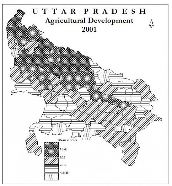
In the present study agricultural development has been considered to be the function of 14 Fig. 2 shows the spatial distribution of region of different level of development. The districts under the very high category (above 0.45 score) constitute two distinct regions in the north-western part of the state. The former region relatively large size includes the districts of Bulandshahr, Rampur, Pilibhit, Shahjahanpur, Moradabad, Kheri and Budaun and the later comprises Saharanpur and Muzaffarnagar districts (Fig. 2). Eleven districts of the state fall under the high level of development (0.15 to 0.45 score) and form a notable region around the periphery of very high level of development in the western and central parts of the state. However, all these districts have the highest value in the case of majority of the selected indicators. The region of moderate level of agricultural development (-0.15 to 0.15) covering about 39 per cent districts of the state and they form a big patch extending from western district down to the southern upland.
The other region of relatively small in size observed is western part. In many of these districts the selected indicators have high value. About 23 per cent districts of the state share low level of agricultural development (-0.45 to -0.15 score) and form two identifiable regions. One relatively large size occurs in the south-western part and the second comprised of eight districts lies in the north-eastern part. The districts of very low grade (below -0.45 score) of agricultural development are scattered sporadically forming a definable region in the state. Here, almost all the chosen indicators are at the low web.
The general picture which emerges from the spatial distribution that overwhelming majority of the north-eastern and southern districts is shown backward in the light of selected variables. The western and central plain districts give an impression of being in a higher side of the scale of development.
6. c) Spatial Patterns of Level of Regional Disparities
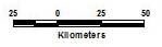
In order to assess the overall level of regional disparities, districtwise z score of 26 indicators having varying nature and characters is calculated separately. A composite index of each districts have been worked out on the basis of these indicators. The interdistricts variations in composite value of z score ranges from -0.96 in Sharawasti to 0.79 in Lucknow districts among the districts of Uttar Pradesh. The districts may be conveniently arranged into five categories of z scores of very high (0.30 and over), high (0.10 to 0.30), medium (-0.10 to 0.10), low (-0.30 to -0.10) and very low (-0.30 and below) z scores fo levels of regional disparities (Table-2). 2
The distribution pattern of level of regional development is uneven all over the districts and presents a very complex picture (Fig. 3). Considering these grades separately, we find that the districts having very high level of regional development constitute three distinct regions, two regions in the western part and the third in the extreme eastern part of the state. All these districts have highest value in case of selected indicators. The high level of regional development districts constitutes two small but distinct regions. One which is large in size lies in the southern part and comprises three districts; Jhansi, Jalaun and Hamirpur. Second which is relatively small in size is found in the eastern part and includes two districts; Azamgarh and Ghazipur which is bit surprising. The other districts of the same grade are scattered in the state. These districts, by and large, rank high in case of selected indicators. The region of moderate level of development covering the largest number of districts (23) and constitute three prominent regions in the state. One lies in the north-western parts that runs from Sitapur in the north to Aligarh in the west and form a longitudinal belt in the state. The second region occurs in south-eastern part and the third in the extreme western part comprising the districts of Muzaffarnagar, Bijnor and Baghpat districts. About 20 per cent districts fall under the grade of low level of regional development. These districts form a number of small regions of which the most prominent one occurs in the north-western part comprising Bareilly, Pilibhit, Kheri and Shahjahanpur districts. The other districts of this grade are scattered over the state. These districts rank low in case of selected indicators. About 16 per cent districts fall under the very low level of development and form two notable regions. One occurs in the north-eastern part and second lies in the north-western part comprising three districts. All these districts stand very low in case of almost all the selected indicators.
The general picture that emerges from this discussion is that the Tarai districts show backwardness in the light of all variables. The western, central and southern districts give an impression of being in a more favourable position. d) Agricultural Development vis-a-vis Regional Disparities
The regional dimensions of agricultural development vis-à-vis regional disparities are shown in Fig. 4. In the key of the map, abscissa represent agricultural development and ordinate the levels of regional disparities. The categories in terms of values are found to be the same for the agricultural development. The districts with reference to composite 'z' score may be arranged into three categories-high (0.15 and over), medium (-0.15 to 0.15 scores) and low (below -0.15 scores).
The figure reveals that about one-third districts of the state lie under the low grade of agricultural development, of which 8 districts are associated with low, two medium and 13 districts high score of the regional disparities. A prominent region of low agricultural development vis-à-vis low level of regional development is found in the north-eastern part of the state. Thirteen districts belong to low level of agricultural development versus high level of development, majority of them form a dominant region in the south-central part. The other districts of this grade are so scattered that they fail to form a definable region in the state. Only two districts i.e., Banda and Deoria have low level of agricultural development with medium level of regional development.
There are 27 districts of the state which come under the medium category of having medium level of agricultural development in which 8 districts show high level, 12 medium levels and 7 low level of regional development. These districts are observed in the eastern and south-central part of the state. A small region of high development coincides with medium level of agricultural development is found in the eastern part to include the districts of Azamgarh, Balli and Ghazipur. The other districts of the same grade are so scattered that they do not form any identifiable region. Two small but distinct regions of medium level of agricultural development versus medium level of regional development constitute in the eastern part of the state. The districts of the medium level of agricultural development versus low level of regional development are scattered sporadically forming a distinct region in the state.
In the high grade of agricultural development (+0.15 z score and over) there are 20 districts, of which three districts-Meerut, Bulandshahr and Fiazabad have high level of development., eight medium level and nine low level of regional development. A dominant region of high level of agricultural development versus low level of regional development is identified in the north-western part of the state. The districts of high grade of agricultural development versus medium level of development are making two separate regions in the study area. One region is located in the western part and another in the central part of the state. In order to investigate, relationships have been sought between agricultural development and other twenty six variables of the seventy districts of Uttar Pradesh. Selection of each variable is based on an ability to develop a rational hypothesis of relationship between the variable and agricultural development. A complete list of variables that affect or may probably affect agricultural development of the district is given in table-4. In order to correlate the agricultural development with 26 independent variables, Pearsonian product moment correlation coefficient (r) has been calculated. The results of correlation coefficient between agricultural development and the variables of levels of regional disparities as shown in Table-4 depict that among the twenty six variables, only one variable (X 26 ) is positively significant at 99 per cent level of confidence with the agricultural development (Y 1 ). However, (X 19 ) No. of livestock population per lakh population and (X 22 ) percentage of electrified villages to inhabitant villages have low degree of positive relationship with agricultural development. Table also shows that four variables are significant at 95 per cent level of confidence in their relationship with agricultural development (Y 1 ). They are: X 2 (Male literacy rate, -0.285), X 13 (No. of Medical (Allopathic) institution per lakh population, -0.273), X 15 (No. of Hospital/Dispensaries (Homeopathic) Medical Services (Govt.) per lakh population, -0.242) and X 23 (Percentage of villages with linked road, 0.293) Only one variable X 23 has direct relationship, whereas the remaining three bears inverse relationship with Y 1. Among the variables, the coefficient of correlation of eleven variables (X 3 , X 4 , X 5 , X 6 , X 7 , X 8 , X 9 , X 10 , X 11, X 17 and X 24 ) records low degree of negative relationships with agricultural development (Y 1 ). This explanation leads to conclusion that literacy rate, urbanization, health facilities, educational facilities and infrastructural facilities are the chief determinants but the magnitudes of their effects are dissimilar.
IV.
7. Conclusion
The general picture which emerges from the spatial distribution of agricultural development shows that overwhelming majority of the north-eastern and southern districts is shown backward in the light of selected variables. The western and central plain districts give an impression of being in a higher side of the scale of development. The above analysis of level of regional disparities clearly indicates that the Tarai districts shows backwardness in the light of all variables. The western, central and southern districts give an impression of being in a more favourable position.
The relationship between levels of agricultural development and levels of regional disparities are marked by substantial increase from west to central and eastern region. Uttar Pradesh is a state where there is a tremendous scope for development in the agricultural sector. Sufficient land is available in the state which could be brought under cultivation and by increasing irrigation facilities, gross crop area can be increased considerably. The districts having low level of regional development should be given top priority so that they may come up at par with developed areas, and the concept of planning with social justice may be fulfilled.


| indicators |
| Category | Composite Score | No. of Districts | Percentage of the |
| Range | Total District | ||
| Very high | > 0.30 | 8 | 11.43 |
| High | 0.10 to 0.30 | 14 | 20.00 |
| Medium | -0.10 to 0.10 | 27 | 38.57 |
| Low | -0.30 to -0.10 | 12 | 17.14 |
| Very Low | < -0.30 | 9 | 12.86 |
| 70 | 100.00 |
| Disparities in Uttar Pradesh, 2001 | ||
| Variables | Definitions | Agricultural Development (Y 1 ) |
| X 1 | Literacy rate | -0.227 |
| X 2 | Male literacy rate | -0.285* |
| X 3 | Female literacy rate | -0.163 |
| X 4 | Population growth (1991-2001) | -0.011 |
| X 5 | Percentage of urban population | -0.007 |
| X 6 | Sex ratio | -0.151 |
| X 7 | Population density | -0.117 |
| X 8 | Schedule Caste population to total population | -0.141 |
| X 9 | No. of JBS & Senior Basic Schools/lakh population | -0.142 |
| X 10 | No. of HSS & Degree Colleges / lakh population | -0.119 |
| X 11 | Educational institute/ Student ratio | -0.016 |
| X 12 | Teacher / Student ratio | 0.029 |
| X 13 | No. of Medical (Allopathic) institution per lakh population | -0.237* |
| X 14 | No. of Beds in Hospitals/ Dispensaries (Allopathic) per lakh | -0.184 |
| population | ||
| X 15 | No. of Hospital/Dispensaries (Homeopathic) Medical | -0.242* |
| Services (Govt.) per lakh population | ||
| X 16 | No. of Doctors per lakh population | -0.224 |
| X 17 | No. of Family welfare clinic / Centres per lakh population | -0.172 |
| X 18 | Percentage of workers engaged in the non-agricultural | -0.096 |
| activities | ||
| X 19 | No. of livestock population per lakh population | 0.204 |
| X 20 | No. of persons engaged in registered factories / Lakh | 0.047 |
| population | ||
| X 21 | Per capita income (at Current Price) | 0.050 |
| X 22 | Percentage of electrified villages to inhabitant villages | 0.178 |
| X 23 | Percentage of villages with linked road | 0.293* |
| X 24 | No. of post office/ Lakh population | -0.067 |
| X 25 | No. of telegraph offices / Telephone exchange/ lakh | -0.076 |
| Population | ||
| X 26 | No. of regulated markets. | 0.395** |