1.
these water resources can alleviate the problem of drought approximately.
One of the management techniques of ground water resources is artificial recharge of basins and determination of the most appropriate place for it. The ground water resources are the largest and most importance reservoirs of drinking water on the earth for human being after glaciers and glacial zones (Freeze, 1979). Since these resources are 99% of whole available drinking water, it is necessary to determine and exploit the ground water (Kouthar, 1986).
Furthermore, it includes 80% of being used resources in arid and semi-arid areas in most countries (Sedaghat, 1994). Due to Iran`s situation in desert and semi-desert area and its average annual rainfall about 250 mm, so there were many ways to prepare drinking water for agriculture, drinking and industry in different parts of country from a long time ago. Therefore, determination and zoning the most appropriate area for artificial recharge of underground aquifers should be considered in this plain.
In recent years, water exploitation has become greater for many reasons such as population growth, industrial development, urbanization growth and consequently increased demand for food products. Hence the rate of exploitation and consumption ground water become greater than recharge of them, in other words input of ground water system is less than its output and system with negative balance sheet has positive feedback and it is collapsing. Thus it is very significant to determine and assign the suitable position for this case.
Water resources management is a set of various management activities aimed at the optimum utilization of water resources and reduction of economical, social and environmental damages and losses. Decision making issue in water resources management is very complex and complicated because of several decision indicators and criteria. Achieving a Introduction owadays, because of uncontrolled exploitation of ground water, water shortage is became doubled. Accurate control and management of N determine purpose, there are a lot of solutions with different priorities for various issues such as environmental, social, organizational and political problems. These necessities leads to use of multiple criteria decision making aimed at selection of best solution among different solutions.
There are several studies on ground water and their artificial recharge all over the world. For example,
M.H.Ramesht ? , Alireza Arab Ameri ? & Mahmood Soltanian ?Author ? : M.A degree in physical geography, department of physical geography, university of isfahan, Iran. E-mail : [email protected] Krishnamurthy et.al (1995Krishnamurthy et.al ( , 1996) ) used RS and GIS techniques to find a suitable position for artificial recharge of ground water in India. Also, they investigated the effects of geomorphologic and geological factors on the behavior of ground water and stated that there is a special unevenness in each area for recharge of ground water. Saraf and Choudhury (1998) used remote sensing capabilities in extracting different layers like land usage, geomorphology, vegetation, and their integration in GIS environment to determine the most suitable area for artificial recharge of ground water. Mahdavi (1997) investigated water management and artificial recharge of ground water in Jahrom city and indicated that controlling usage and recharge of water tables by the watershed management is the main management technique. Abdi and Ghayoumian (2001) prioritized the suitable areas for storing surface water and reinforcing ground water based on geophysics data, land usage, topography, their integration and analysis in GIS environment. KiaHeyrati (2004) Mianabadi and Afshar (2008) investigated and ranked the project of water supply in Zahedan using three methods: Induced Ordered Weighted Averaging (IOWA), Linear Assignment and TOPSIS methods, and then they compared the findings of these methods with the results of adaptable planning method (Mianabadi, 2008). Limon and Martinez (2006) used Multi Attribute Utility theory for optimum allocation of agriculture water in north of Spain (Limon, 2006). Ahmadi et al (2002) used multiple criteria decision making to rank different projects of refining agriculture water to reuse them (Ahmadi, 2002). Also, Anand Raj and Kumar (1996) ranked management options of river basin by ELECTRE method (Anand, 1996).
The purpose of this is zoning the best areas for artificial recharge of underground aquifers in Zarand-Saveh watershed using the effective factors in nurturing underground water tables by ELECTRE method, linear assignment and GIS techniques. In other words, this investigation attempts to find and zone the most suitable area for artificial recharge of underground aquifers using the analysis of effective parameters on soil penetrability and recharge of underground water tables by ELECTRE method, linear assignment and preparing its raster layers in the environment of soft ware Arc GIS 9.3.
2. II.
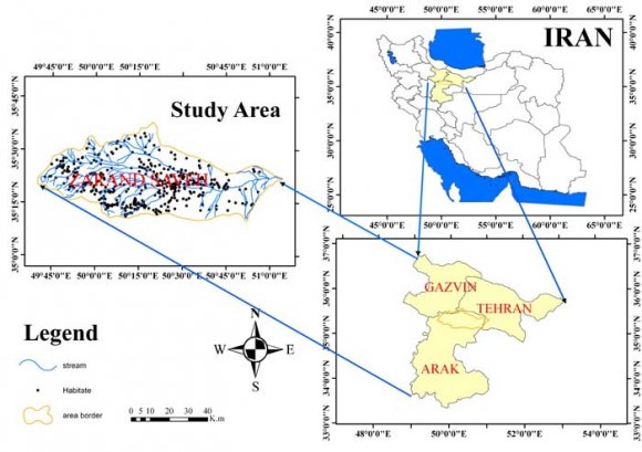
Methods and Materials a) Mathematical situation of studied area Being situated in the north part of central province, Saveh province is bounded by 34º, 45' latitude to 35º, 34' north latitude and 49º, 15' to 50º and 56' longitude. It has access to Ghazvin province in north, to Tafresh and Qom provinces in south, to Tehran province in east and to Hamedan province in west. Globally, Saveh is located at 1250 meter height above sea level and its extent is 1027 square kilometers.
3. Methods
Firstly, studied area was investigated by the satellite images of Google Earth and its limitations were determined. Then digital elevation model of area was separated from its digital elevation model in Iran in the environment of soft ware GlOBAL MAPER and the output was received. Required data layers for zoning in the environment of software Arc GIS 9.3 was prepared as following:
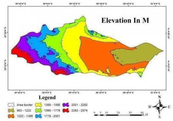
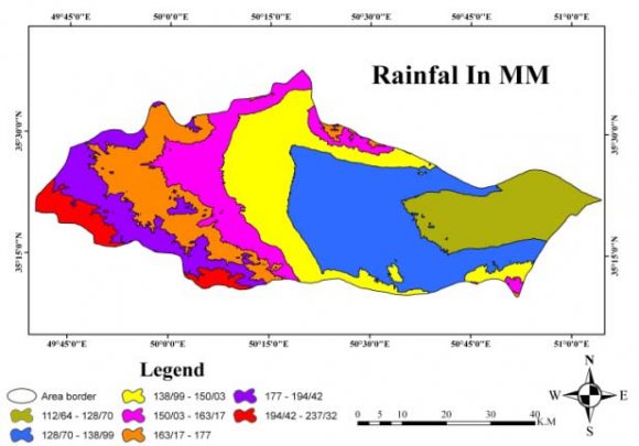
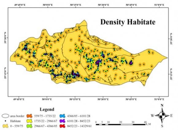
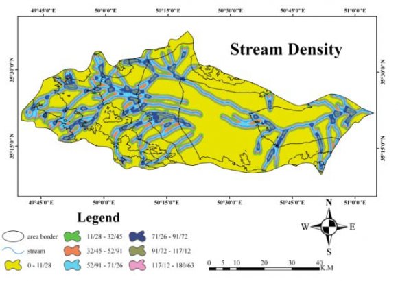
First, digital elevation model classified in to 7 elevation classes based o natural breaks in the heights of the area (figure2). Mentioned classes represent the studied zones in the area and subsequent calculations were done in each of these classes. Slope layer prepared base on digital elevation model o the area by surface analyses tool in 3D analyses. There were different processes to prepare drainage density layer and habitual density such as digitizing main and minor waterways layers on the topographical map1:50000 of the area, digitizing main and minor fault on geological map 1:100000 of area and density tool in Spatial Analyses.
Iso-Precipitation layer prepared by interpolating method like cringing technique and linear relationship between rain-height using Interpolate tools in 3D analyses (Figure 2 to 8).
Second, the investigated criteria for each height zones were calculated (Table1) and their layers prepared separately. After achieving a few numbers in each layer, the numbers were analyzed by ELECTRE and Linear Assignment methods and mentioned zones prioritized to select the most appropriate area for artificial recharge of underground watersheds in the studied area.
4. a) Theoretical principles of ELECTRE method and Linear Assignment
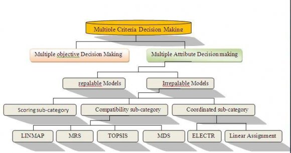
In recent decades, several researchers attempt to use Multi Criteria Decision Making (MCDM) in complex and complicated decisions. These decision methods divide into two parts;
5. MODM = Multi Objective Decision Making 2. MADM = Multi Attribute Decision Making
Multi Criteria Models use to select the best options. Evaluative Models for MADM classify into two models; 1. Compensatory Model 2. Non-Compensatory Model Non-compensatory model includes methods which don`t need to achieve data from DM and lead to objective answer. Exchanging between indictors is permitted in Compensatory model. It means that for example, a weakness in a indicator may be compensated by option of other indicator. Electrical Method is a type of available methods in Compensatory Models. In this method whole options evaluate by nonranked comparisons. All stages of this method are established based on coordinated and uncoordinated sets and thus this method is known as ''Coordination Analysis''. Banayoun established the Electrical Method and Delft, Nijkamp, Roy and their colleagues developed it. In Electrical method, the concept of domination uses implicitly. In this method, options are compared in pairs, then dominant and weak (dominant and defeated) options determined and weak or defeated options omitted (Roy, 1991;49-73).
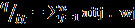
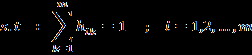
Linear Assignment is one of the Multi Criteria Decision Making combines qualitative and quantitative indicators, weights criteria based on their importance and helps decision makers to select the best options at the same time. In this method, supposed options are ranked based on their points in each available indicator and then the final rank of the options determined by the Linear Compensatory Process. The situation of these two models show among the other Multi Criteria Decision Making (Figure2).solution process doesn`t need to scale down the quantitative and qualitative indicators. If option i were in rank t in indicator j, then ?itj= 1 otherwise it would be ?itj. 4. The following assignment problem is solved with variables (0, 1 hit) in order to determine the final priority of options.
(
(3)
6. Ranking Options
In the final stage, the options are ranked.
c) Problem-Solving process in ELECTRE method 1. Establishing Decision Making Matrix: According to the criteria and numbers of options and evaluation of whole options for the different criteria, Decision Making Matrix develops as follow;
In which the Function of Xij (i = 1,2, ... ...., M) is in relation to the criteria I j (j = 1,2,3, ... ..., n).
7. Scale down the Decision Making Matrix:
In this stage, all criteria with different dimensions is changed into the dimensionless criteria and matrix R defined as follows. There are several methods to scale down, but generally the following equation used in electrical method (Tille: 2003, 19-21).
8. Determining Weighted Matrix of criteria:
As you can see, Weighted Matrix (W) is diagonal matrix in which the elements on main diameter are not zero and amount of these elements equal to importance coefficient of the related vector.
9. Determining Weighted Normalized Decision Matrix:
Weighted Normalized Decision Matrix is obtained by multiplying Scale down Decision Making Matrix into the Weighted Matrix of criteria.
10. Establishing agree and disagree criteria set
The criteria set J = (1, 2... m) divides into two subsets; agree and disagree for each pair of options e, k (k, e = 1,2, ...., M, k # e) . Agree Set (SKe) is a set of criteria in which option K is preferred to option e. and its complementary set is the opposite set (IKe) in mathematical language;
(5) (6)
11. Establishing Agree Matrix:
To establish agree matrix, its elements, agree indicators, should be calculated. Agree indicator is sum of weight of criteria in agree set. Thus, indicator Cke is between option k and option e equals to (Roy, 1991, 49-73):
(7) For total normalized weights equals 1 so:
(8)
Agreement represents the superiority of options k on option e which its amount changes in the range of zero to one (0-1). After calculating agree indicator for all options, matrix which is a m * m matrix is defined as follows. Generally, this matrix is not symmetrical. It noticed that the data including in agreement matrix, are different from data in opposite matrix and in fact these data are completed each other. The difference between the weight is developed through agreement matrixes, while the difference between determined values is obtained throug h opposition matrix.
12. Establishing agree dominant matrix:
In the sixth step, it indicated how to calculate agreement indicator Cke. Now there is a determined amount for agreement indicator in this step which is called agreement threshold . If Cke is larger , option k is preferred on option e, otherwise it is not. Agreed threshold is calculated by the following equation (Roy, 1991, 49-73): (10) Agree Dominated Matrix (F) is developed based on the amount of agreement threshold and its elements determined in the equation bellow (Vami, 1992). (11) 9. Establishing Opposed Dominance Matrix : Opposed Dominance Matrix (G) is establ ished the same as Agree Dominated Matrix. First, decision makers should express opposite threshold which is for because opposite amount (disagreement) expresses superiorities dimension of option k on option is acceptable. In contrast, if (dke) were larger than , opposite amount would be very grea t and it would not be ignored. Thus, Opposed Dominance Matrix is defined as follows (1991, 49-73): (13) Each element in the matrix (G) shows the dominant relationship between options.
13. Establishing Final Dominant Matrix:
Final Dominant Matrix (H) is developed after multiplying each element in Agree Dominated Matrix (F) into elements in Opposed Dominance Matrix (G) (Roy, 1991, 49-73). (14) 11. Removing less satisfaction options and selecting the best option: Final Dominant Matrix (H) indicates detail preferences of options. For example, when amount of hke equals 1, it means that option k is preferred on option e in both agree and disagree situation (it means its preference is larger than the agree threshold and its opposite or weakness is less than disagree threshold), but option k may be dominated by other options yet. The options should be ranked in a way that the more dominated options are selected than the more defeated one.
Determining the importance coefficient of options than the other, criteria are compared in pair by time suggested method. The amount of disagreement indicator changes from zero to one. After calculating disagree indicator for all options, matrix which is a m * m matrix is defined as follows. Generally, this matrix is not symmetrical.
14. Determining Opposite Matrix
Disagreement indicator (opposite) is described as follows (Roy: 1991, 49-73): After the formation of paired comparison matrix, relative weights of criteria can be calculated. There are different methods to calculate the relative weight based on paired comparison matrix. The most important ones are the "least squares method, least squares logarithmic example the mean of opposite indicators (disagreement) (Roy, 1991, 49) -73): (15) method, special vector method and approximate method. The special vector method is the most accurate one. In this method, Wi is determine in the equation12: A×W=?maxW the greatest value of ? in equation ( 13), the amount of wi is calculated. (2001, 315: Saaty). ( 16)
IV.
15. Research Findings
The results of ELECTRE and Linear Assignment methods to find the most suitable area for artificial recharge of groundwater aquifers of Zarand-Saveh watershed showed in figures ( 2) to (8) and tables (3) to (12). Therefore, a matrix is formed with rank (49) for data matrix, with 7 alternatives (height zones) and 7 related indicators (rainfall, stream density, habitual density, extent, land area facies, slope, height) (Table 3). substitutions out of different elements and deciding about them is important is significant in environmental planning and management. In other words, it is necessary to use suitable methos which are combined different indicators in order to achieve better results and to do the best job for environmental planning and management.
1 0 0 0 0 0 0 1 2 1 0 0 0 0 1 1 3 1 1 0 0 0 1 1 4 1 1 1 0 0 1 1 5 1 1 1 1 0 1 1 6 1 0 0 0 0 0 1 7 1 0 0 0 0 0 0 ( D D D D ) b1 0 0 0 0 0 0 0 2 1 0 0 0 0 0 1 3 1 1 0 0 0 1 1 4 1 1 1 0 0 1 1 5 1 1 0 0 0 1 1 6 1 0 0 0 0 0 1 7 1 0 0 0 0 0 01 0 0 0 0 0 0 0 2 1 0 0 0 0 0 1 3 1 1 0 0 1 1 1 4 1 1 1 0 1 1 1 5 1 1 0 0 0 1 1 6 1 0 0 0 0 0 1 7 1 0 0 1 0 0 00 0 0 0 1 0 0 0 1 0 0 0 2 0 0 0 0 0 0 1 3 0 0 0 0 0 1 0 4 0 0 0 0 1 0 0 5 0 0 1 0 0 0 0 6 0 1 0 0 0 0 0 7This study aimed at ranking the water resources potential in Zarand-Saveh watershed by two methods; ELECTRE method and Linear Assignment. ELECTRE method is one of the Multi criteria decision making which can compound the quantitative and qualitative criteria, weight each criterion based on its importance and help decision makers to select the best option at the same time.
V.
16. Discussion and Conclusion
Having Systematic attitudes toward geography as a science distribution indicates that geography is depending on Mathematical Sciences (Shakoeei, 1999, 43). Generally, model ( 1) is a shematic but accurate description about a system which is corresponded with its previous behavior and therefore, there is hope that it will be used to predict the future behavior of the system (Hekmat-Nia and Moosavi, 2007, 29).
In recent decades, researchers have used Multi Criteria Decision Making in complex and complicated decisions. In these models, several criteria are used to measure instead of desirable criteria (Taherkhani, 2008, 62). Nowadays, prioritizing and selecting appropriate Electrical method is one of the available methods in compensatory methods. In this method, all options are analyzed and evaluated by non-ranked comparisons. Whole stages of this method are based on coordinated and uncoordinated sets and thus it is called ''coordination analysis''. The results and findings show that zone (4) dominated (5) times and defeated (1) time,so it is located in the first rank with (4) points and is the most suitable zone for artificial recharge. In contrast, zone (1) defeated (6) time and dominated no time, therefore it is located in the last rank with (-6) points and is not the most suitable zone for artificial recharge. And, zones (3, 5, 2, 6, 7) dominated (4, 4, 2, 2, 1) times and defeated (5, 4, 2, 2, 4) and located in other ranks with (-4, -2, -2, 2, 2, 2) points respectively. Also, zones (7, 6, 2, 1) should be omitted because their defeated times are more than dominated times. And in Linear assignment, zone (3) is located in the first rank, zone (8) in the last rank and zones (7, 2, 6, 5, 4) in other ranks respectively.




| Numerical values | Preferences (judging verbal) | |||
| 9 | Extremely preferred | |||
| 7 | Very strongly preferred | |||
| 5 | Strongly preferred | |||
| 3 | Moderately referred | |||
| 1 | Equally preferred | |||
| ? 2 | ? 4 | ? 6 | 8 | Intervals between strong preferences |
| Regions | Materials | Precipitation | Stream density | Slope | Habitual density | Elevation | area |
| 1 | 1 | 121.29 | 90.31 | 13.28 | 4975.46 | 1092.5 | 484.85 |
| 2 | 5 | 134.22 | 63.91 | 22.09 | 5696.15 | 13.5 | 958.1 |
| 3 | 9 | 144.66 | 76.99 | 26.71 | 3268 | 1435.5 | 695.27 |
| 4 | 9 | 157.28 | 79.115 | 31.68 | 7164.8 | 1672 | 461.46 |
| 5 | 7 | 169.62 | 85.42 | 49.86 | 5911.25 | 1889.5 | 478.64 |
| 6 | 3 | 185.58 | 62.23 | 48.73 | 4692.22 | 2141.5 | 363.41 |
| 7 | 1 | 214.41 | 61.19 | 36.61 | 3163.1 | 2628 | 149.57 |
| Regions | Materials | Precipitation | Stream density | Slope | Habitual density | Elevation | area |
| 1 | 0.0636 | 0.2801 | 0.4553 | 0.1433 | 0.3646 | 0.2378 | 0.3245 |
| 2 | 0.3181 | 0.3099 | 0.3222 | 0.2384 | 0.4175 | 0.0029 | 0.6412 |
| 3 | 0.5727 | 0.3340 | 0.3882 | 0.2883 | 0.2395 | 0.3124 | 0.4653 |
| 4 | 0.5727 | 0.3632 | 0.3989 | 0.3420 | 0.5251 | 0.3639 | 0.3088 |
| 5 | 0.4454 | 0.3916 | 0.4307 | 0.5382 | 0.4332 | 0.4112 | 0.3203 |
| 6 | 0.1909 | 0.4285 | 0.3137 | 0.5260 | 0.3439 | 0.4661 | 0.2432 |
| 7 | 0.0636 | 0.4951 | 0.3085 | 0.3952 | 0.2318 | 0.5719 | 0.1001 |
| Criteria | Materials Precipitation | Stream density | Slope | Habitual density | Elevation | area | Wij | ||
| Materials | 1 | 3 | 5 | 5 | 7 | 7 | 9 | / 0 | 3868 |
| Precipitation | 0.33 | 1 | 3 | 5 | 5 | 7 | 7 | / 0 | 2349 |
| Stream density | 0.2 | 0.33 | 1 | 3 | 5 | 7 | 7 | / 0 | 1585 |
| Slope | 0.2 | 0.2 | 0.33 | 1 | 3 | 5 | 7 | / 0 | 1028 |
| Habitual density | 0.14 | 0.2 | 0.2 | 0.33 | 1 | 3 | 5 | / 0 | 0603 |
| Elevation | 0.14 | 0.14 | 0.14 | 0.2 | 0.33 | 1 | 3 | / 0 | 0353 |
| Area | 0.11 | 0.14 | 0.14 | 0.14 | 0.2 | 0.33 | 1 | / 0 | 0214 |
| Inconsistency rate: 0/0252 (due to being less than 0/1 compatibility matrix indices are acceptable) | |||||||||
| Regions | Materials Precipitation | Stream density | Slope | Habitual density | Elevation | area | |
| 1 | 0.0000 | 0.1940 | 0.2189 | 0.1799 | 0.1799 | 0.2404 | 0.6266 |
| 2 | 0.8059 | 0.0000 | 0.0820 | 0.0215 | 0.0215 | 0.6266 | 0.6266 |
| 3 | 0.7810 | 0.9179 | 0.0000 | 0.4077 | 0.4077 | 0.5661 | 0.6266 |
| 4 | 0.8200 | 0.9784 | 0.9784 | 0.0000 | 0.4467 | 0.6266 | 0.6266 |
| 5 | 0.8200 | 0.9784 | 0.5922 | 0.5532 | 0.0000 | 0.7294 | 0.7294 |
| 6 | 0.7595 | 0.3733 | 0.4338 | 0.3733 | 0.2705 | 0.0000 | 0.7294 |
| 7 | 0.7595 | 0.3733 | 0.3733 | 0.3733 | 0.2705 | 0.2705 | 0.0000 |
| Regions | Materials Precipitation | Stream density | Slope | Habitual density | Elevation | area | |
| 1 | 0 | 1 | 1 | 1 | 1 | 1 | 1 |
| 2 | 0.214494 | 0 | 1 | 1 | 1 | 0.601495 0.442481 | |
| 3 | 0.054111 | 0.109532 | 0 | 1 | 0.522695 | 0.165727 0.192437 | |
| 4 | 0.045479 | 0.072698 | 0.194701 | 0 | 0.410479 | 0.128322 0.157619 | |
| 5 | 0.026487 | 0.140366 | 1 | 1 | 0 | 0.088066 0.164765 | |
| 6 | 0.456288 | 1 | 1 | 1 | 1 | 0 | 0.318163 |
| 7 | 0.460453 | 1 | 1 | 0.1028 | 1 | 1 | 0 |
| Regions | Materials Precipitation | Stream density | Slope | Habitual density | Elevation | area |
| Regions | Materials Precipitation | Stream density | Slope | Habitual density | Elevation | area | |
| 1 | 0.0246 | 0.0658 | 0.0721 | 0.0147 | 0.0221 | 0.0085 | 0.0070 |
| 2 | 0.1229 | 0.0728 | 0.0510 | 0.0245 | 0.0253 | 0.0001 | 0.0138 |
| 3 | 0.2212 | 0.0785 | 0.0615 | 0.0296 | 0.0145 | 0.0111 | 0.0100 |
| 4 | 0.2212 | 0.0853 | 0.0632 | 0.0352 | 0.0318 | 0.0130 | 0.0066 |
| 5 | 0.1720 | 0.0920 | 0.0682 | 0.0553 | 0.0262 | 0.0146 | 0.0069 |
| 6 | 0.0737 | 0.1007 | 0.0497 | 0.0541 | 0.0208 | 0.0166 | 0.0052 |
| 7 | 0.0246 | 0.1163 | 0.0489 | 0.0406 | 0.0140 | 0.0204 | 0.0022 |
| Regions | Materials Precipitation | Stream density | Slope | Habitual density | Elevation | area |
| Difference | Number being defeated | Rule number | Regions |
| -6 | 6 | 0 | 1 |
| -2 | 4 | 2 | 2 |
| 2 | 2 | 4 | 3 |
| 4 | 1 | 5 | 4 |
| 2 | 2 | 4 | 5 |
| -2 | 4 | 2 | 6 |
| -4 | 5 | 1 | 7 |
| b) Problem Solving Matrixes in Linear Assignment Method | |||
| D D D D ) | |||||||
| ( | |||||||
| Regions | Materials Precipitation | Stream density | Slope | Habitual density | Elevation | area | |
| 1 | 2 | 121.29 | 90.31 | 13.28 | 4975.46 | 1092.5 | 484.85 |
| 2 | 5 | 134.22 | 63.91 | 22.09 | 5696.15 | 1300.5 | 958.1 |
| 3 | 9 | 144.66 | 76.99 | 26.71 | 3268 | 1435.5 | 695.27 |
| 4 | 8 | 157.28 | 79.115 | 31.68 | 7164.8 | 1672 | 461.46 |
| 5 | 7 | 169.62 | 85.42 | 49.86 | 5911.25 | 1889.5 | 478.64 |
| 6 | 3 | 185.58 | 62.23 | 48.73 | 4692.22 | 2141.5 | 363.41 |
| 7 | 1 | 214.41 | 61.19 | 36.61 | 3163.1 | 2628 | 149.57 |
| Regions | Materials Precipitation Stream density | Slope | Habitual density | Elevation | area |
| Regions | first | Second | third | Fourth | Fifth | Sixth | Seventh |
| 1 | 3 | 1 | 1 | 1 | 0 | 0 | 1 |
| 2 | 0 | 2 | 1 | 1 | 2 | 1 | 0 |
| 3 | 1 | 1 | 2 | 1 | 2 | 0 | 0 |
| 4 | 1 | 1 | 1 | 4 | 0 | 0 | 0 |
| 5 | 0 | 1 | 1 | 0 | 2 | 2 | 1 |
| 6 | 1 | 1 | 1 | 0 | 0 | 4 | 0 |
| 7 | 1 | 0 | 0 | 0 | 1 | 0 | 5 |
| Regions | first | Second | third | Fourth | Fifth | Sixth | Seventh |
| 1 | 0.2968 | 0 | 0.215 | 0.0605 | 0 | 0.3862 | 0.2349 |
| 2 | 0.215 | 0.1384 | 0.0605 | 0.3862 | 0.1584 | 0.2349 | 0 |
| 3 | 0.3862 | 0.0215 | 0.1384 | 0.1584 | 0.2349 | 0.0605 | 0 |
| 4 | 0.0605 | 0.3862 | 0.1584 | 0.3948 | 0 | 0 | 0 |
| 5 | 0 | 0.2189 | 0.6211 | 0 | 0.0571 | 0 | 0.1028 |
| 6 | 0 | 0.2349 | 0 | 0 | 0.4467 | 0.3183 | 0 |
| 7 | 0.2349 | 0 | 0 | 0 | 0.1028 | 0 | 0.6622 |
| Points | ||
| Regions | ||
| 0 | 0 | 1 |
| D D D D ) | |||||||
| ( | |||||||
| Regions | 1 | 2 | 3 | 4 | 5 | 6 | 7 |
| Rated | Seventh | Second | first | Fourth | third | Fifth | Sixth |
| Rated | Materials | Precipitation | Stream density | Slope | Habitual density | Elevation | area |
| first | 3 | 7 | 1 | 1 | 4 | 1 | 2 |
| Second | 4 | 6 | 5 | 2 | 5 | 2 | 3 |
| third | 5 | 5 | 4 | 3 | 2 | 3 | 1 |
| Fourth | 2 | 4 | 3 | 4 | 1 | 4 | 4 |
| Fifth | 6 | 3 | 2 | 7 | 6 | 5 | 5 |
| Sixth | 1 | 2 | 6 | 6 | 3 | 6 | 6 |
| Seventh | 7 | 1 | 7 | 5 | 7 | 7 | 7 |