1. I. Introduction
here is substantial amount of academic literature on the energy consumption. However, much of academic research seems to be narrowly focused, covering only a few economies and factors. Moreover, the academic literature is obscure and scarce on whether globalization has amplified or reduced the consumption of traditional fossil fuels to satisfy expansion in energy demand. Therefore, here we venture to bridge the gaps available in the academic literature, by providing an empirical framework that encompasses the change in fossil fuels consumption for 66 developing countries that result from globalization.
In this paper, globalization comes in many flavors, including economic, political and social elements. Because globalization is a multidimensional phenomenon, we focus on different aspects of globalization to provide the empirical modeling that captures volatility in energy need that arise from globalization effect. Some academic literature suggests that globalization has made the world into a single system and connected countries through the exchange of information, trans border maintenance of produced technology and international technological partnership. Some argue that this flow leads to technological innovation which in turn leads to efficiency and cost-cutting. Thus this paper focuses on whether globalization has amplified the consumption of traditional energy or if there is a successive switching towards clean and renewable energy sources through the attainment of technological efficiency.
We organize the remainder of the paper as follows. Section 1 gives information of how energy consumption has evolved recently in developing economies. It also provides a brief methodology on globalization. Section 2 delivers the academic literature related to globalization and its impact on energy demand. In section 3 we give a brief description of the dataset, and present the results of various statistical specifications and findings. The last section provides findings and discussions.
2. II. Theoretical Framework
The emerging economies are increasingly becoming substantial actors in international commercial energy demand. Their share of the total energy use has magnified abruptly in the last decades, from 12 percent of worldwide energy use in 1970 to 57 percent in 2014. Notwithstanding that their per-capita is much lower than that of the industrialized countries; developing countries accounted for more than one-half of the total growth in global energy use since 1970 (see Table 1). Figure1 displays the sources of energy for the developing group of countries. The developing group mostly uses coal and oil to meet their energy demand.
Its worth to note that, much of the coal is used in China and India only. Most of the developing countries use oil as a primary source of energy supplies.
Source: BP statistical review of world energy, 2014 2). China alone accounts for more than 22 percent of the global l energy consumption and 40 percent of commercial energy use among developing countries. China's future energy course will potentially change the energy flows in the region and globally.
At the other end of the scale there is a number of the emerging group that together, that justify only a moderate portion of worldwide energy use. For example, countries of South Africa, consume less than 1 percent of overall fossil fuels (see Table 2).
3. Oil 30%
4. Natural Gas 19%
Coal 42%
Nuclear Energy 2%
5. Hydro electric 6%
Renewables 1% To analyze in more details how the energy intensity in developing countries changed as a result of the globalization, we focus on different aspects of globalization. Accordingly, to capture the globalization power of developing countries, we use the globalization index Konjunktur for schungs stelle (KOF) developed by the Swiss Economic Institute (Dreher 2006(Dreher , 2008)). The KOF index displays the power of globalization in three dimensions: economic globalization, which estimates business flows with an assumption for confinements to capital and trade; social globalization, which accumulates the dissemination of information, population, ideas, and images and; political globalization, which shows the diffusion of government policies. These three indices are weighted by the weights of variables making up these indices. The weights such as 36%, 37% and 27% are allocated between economic, social and political dimensions of globalization, respectively. These weights are computed based on the values of sub-indices composing the indexes. The three indices are always between 1 and 100, with a greater index indicating on a higher degree of globalization.
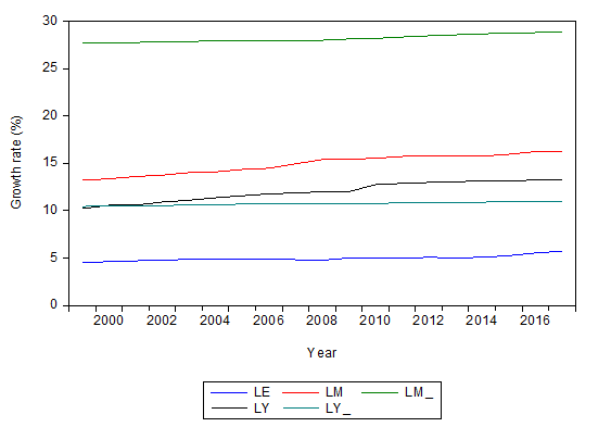
Figure 2 illustrates the trend of globalization index for some developing countries. For these, the overall globalization score together with its sub-variables has considerably ameliorated between 1971 and 2014time span. The data suggests that the overall globalization index of 83.64 for Singapore is the highest among developing countries. For Thailand, the overall globalization index has also been significantly improved reaching 70.76 in 2014.
6. Source: World Bank Data Extract
7. III. Literature Review
There is surprisingly very scarce literature record connecting globalization and energy demand. To my best knowledge, only one empirical study on energy consumption and globalization exist in the literature. The 2012) and others on globalization and its effect on different macroeconomic frames have been used in this paper.
We do not venture to present such a review here, but do use these studies to avoid overlapping and place my analysis within the literature.
8. IV. Empirical Analysis
The empirical investigation covers annual time series for the 66 developing economies.. Annual data on energy consumption and income are extracted from World Development Indicators. The income time series considered in the model as a control variable connecting energy use and globalization. I extract the data on the three globalization indices from KOF Globalization Index (2013). The length of an analysis depends on the availability of data; therefore, the empirical period is between 1998-2014. In the statistical analysis, we use natural logarithms of all variables.
9. a) The stationarity testing
The first estimation of stationarity was conducted with Levine, Lin and Chu (2002) test. According to if the first order serial correlation coefficient is ?, then the null hypothesis is that H 0: ? i =1 for i=1?.
N, in contrast to homogeneous assumption H 1 1 :-1< ? i = ?<1 for i=1?. N. Therefore, according to the second hypothesis the ? is expected to be equal in all terms, by keeping them uniform throughout cross-sectional units as follows:
??? ???? = (?? ?? ? 1)?? ???? ?1 + ? ?? ???? ??? ???? ??? + ?? ?? ?? =1 ?? ???? ?? ???? + ?? ???? , ?? = 1,2,(?? ?? ? 1) = 0 ð??"ð??"ð??"ð??"ð??"ð??" ?? = 1 ? . . ?? , then ?? = ? ? ?? ???? ð??"ð??" ???? ?1 ?? ??=?? ??+2 ?? ??=1 ? ? ð??"ð??" ???? ?1 2 ?? ??=?? ??+2 ?? ??=1. Im, Pesaran and Shin (1997) unbrace the hypothesis of the LLC test and allow first-order serial correlation coefficients to change across regions as follows:
?? ? = ?????? ? ???(??? )? ?????ð??"ð??" (??? ), where
?? ? = 1 ?? ? ?? ??, ?? ??=1the terms ????ð??"ð??"(?? ? ) and ??(?? ? ) are the variance and mean of individual ?? ?? statistic, and ?? ? statistic approximate to a standard normal distribution. Hadri (2000) estimates a Lagrange ratio with the residuals obtained from the following equation ?? ???? = ?? ???? ?? ???? + ?? ???? ??????? ?? = 2,3 for i=1,??,
N. ???? = 1 ?? ? 1 ?? 2 ? ?? ???? 2 ?? ??=1 ?? ? ?? 2 ?? ??=1, where
?? ???? = ? ?? ???? ?? ?? =1and ?? ? ?? 2 is the long-run variance estimate of disturbance terms. Table 3 exhibits the panel unit root estimators. At a 5% significance level, except for the IPS statistic for income and energy use variables with individual intercept and individual intercept and trend, other estimators significantly support that five series are stationary. Using these results, I test the time series with the error components model for evidence of the relationship.
10. Table 3: Unit root test results
11. b) The Error Components Model
In this paper, we use the error components model because there is no correlation between the individual effects and the other regressors. This model allows the intercepts for each cross-sectional unit to arise from a common intercept ?? . Moreover, it is assumed that the global intercept is the same for all cross-sectional units and over time as follows: ???? ???? = ?? + ???????? ???? + ?????? ???? + ?????? ???? + ?????? ???? + ?? ???? , ?? ???? = ?? ?? + ?? ???? , where ?? ?? is a random variable with zero mean and constant over time but varies cross-sectionally. A random variable determines the arbitrary deviation of individual unit's intercept terms from the common intercept term ?? and is independent of each observation Where ???? and ???? are fixed and random estimators, and ??????ð??"ð??" is asymptotic variance-covariance matrices obtained from fixed and random estimations. This test is used in this study to decide which model is statistically appropriate. According to the test results at 5 % significance level, the null hypothesis can be accepted (see Table 5). We conclude that the error component is an appropriate model for the small distance.
12. ??
, where ?? ???? = ??? ???? ? ?? ? ?? ? , in this equation ?? ???? is j observation of X variable in group i and n is the number of observations and g is a number of units. From the probability estimators, at 5% significance level I concluded that the error terms are heteroscedastic (see Table 6). If the errors don't have a constant variance their mean value is roughly constant however their variance is rising systematically with the values of dependent variables. as proposed by Bhargava, Franzini and Narendranathan (1982), where ???= ??????ð??"ð??"(?? ?? ?? ?? ? )??? ? ???? ? ? , ?? ? is obtained from the estimation by the pooled least squares model ?? ? = ?? ? ?? + ?? .The estimators are indicating on the availability of positive, consistent correlation in the residuals (see Table 7). This condition shows that the standard error terms can inflate the model as they will be biased downwards relative to the true standard errors. Therefore, the test will belittle its true value with underestimating of the true error variance. We diagnose that the error component model with time effects has heteroscedasticity and serial correlation. Therefore, to eliminate the deviations from assumptions, I use Arellano (1987Arellano ( , 1993) )
standard errors technique ????ð??"ð??"??? ?? = ???1 ????? ?? ???1 (?? ? ??) ?1 (? ?? ?? ? ?? ??=1 ?? ?? ? ?? ? ?? ? ?? ?? )(?? ? ??) ?1where ??and ?? are a number of groups, ?? ? ?? is i residual in group j. The Table 8 shows the test results. The results show that the model and some coefficients are statistically significant. Moreover, the test displays 36% explanatory power, indicating that dependent variables can explain 36% of the variation in energy use.
13. c) Vector autoregressive model
We present a VAR model for energy use for a group of n time series ?? ?? = ?? 1?? , ?? 2?? , . . , ?? ???? , as follows (Ciccarelli and Canova, 2004Canova, ,2007Canova, , 2009Canova, , 2013)):
?? ???? = ?? 0?? (??) + ?? 1 (??)?? ???1 + ?? 2 (??)?? ?? ?2 + ? + ?? ?? (??)?? ??,???1+ ?? ?? (??)?? ???1 + ?? ?? where ?? ???? is the vector of dependent variable. The advantage of VAR analysis is that it can be extended to over two and more variables. ?? ???1 is the vector of exogenous variables (if present). ?? 0?? (??) are the deterministic components of the time series (constant terms, deterministic polynomial in time and seasonal dummies). Under the assumption of heterogeneity across units ?? ?? (??) and ?? ?? (??) are polynomials in the lag operators. We estimate operators under homogeneous panel VAR model Mignon 2013, 2015). ?? ?? is evenly and independently disseminated white noise with zero mean. VAR panel analysis includes only the variables that proved to be statistically significant in panel data analysis.
Before conducting impulse response analysis, we tested the stationarity of the VAR model. From the figure, we found that all roots reside within the integer circle and are lower than one (see Figure 3). This result indicates on the stationarity of the VAR model. on the VAR model impulse response analysis shows the destabilization experienced by the variables in response to shocks that arise within other variables. The results from impulse response analysis show that the impact of social globalization on energy use will work till seven lags lengths after which the shocks will die away (see Figure 4). The key question we are interested in is whether the change in globalization can explain the energy demand in developing countries. With this question in mind, we constructed error components estimators and carried out an impulse response analysis. As a result of these analyses, we found that economic and political globalization processes don't have an impact on energy demand in developing countries. On the other hand, the error components estimators indicate on the fact that among three broad globalization dimensions only social globalization has a statistically significant impact on traditional energy consumption. Social globalization reveals 21.7 % of the change in energy consumption. The coefficient of social globalization is statistically significant, and its effect is negative. That is a 1% increase in globalization diminishes conventional energy use by 21.7 %. This result is very important, because the literature is still ambiguous on the effect of globalization on conventional energy demand. The coefficient of the income variable is also significant, and its effect is negative. This suggests that the increase in income by 1 % decreases traditional energy demand by 11 %. Indeed, the affluent industrialized countries with the highest income per capita decrease the share of traditional energy and increasingly implement the large scale and costly energy projects on renewable energy technology.
A similar pattern emerges from impulse response analysis. The impulse response functions show that energy consumption responds negatively to the increase in social globalization. The functions also show that the energy use responds negatively to the increase in demand.
Although it is an indisputable fact that there are a lot of debates and opinions on globalization across the world, it is widely accepted that globalization fosters trading and business performance by means of rise in foreign direct investment and the transfer of progressive technology from developed nations to developing countries. In particular, social globalization which accounts for the proliferation of ideas, skilled employees and know-how is expected to have a tremendous benefit to developing countries and increase use of clean and renewable energy sources through the attainment of technological efficiency.
The estimations show that a 1% increase in globalization diminishes energy use by 21.7 %. If globalization increased globally, then the traditional energy use in developing economies should have been decreased. However, the use of traditional energy in developing countries has risen steadily from 4911.66 million tons in 1970 to 12988.85 million tons in 2014. Their share of the entire energy demand in 2014 accounted for more than half of the total increase in worldwide commercial energy use. This controversial result can be explained by two phenomena. Firstly, globalization together with income accounts for 36% and globalization alone accounts for 21.7% change in energy demand. However, there are other factors that affect the energy demand and the pace of change of these factors may have been greater than increase in globalization. In other words, the negative impact from the change in other factors may outweigh the benefits from the increase in globalization causing traditional energy demand to increase.
Secondly, this contradictory result may indicate the trend of globalization in reverse. Some countries benefit from globalization process, but probably there is an uneven development of globalization in clean energy consumption around the world. With normal functioning of social globalization, the ideas, skilled people, information and technology transfer very quickly from advanced economies to developing world leading to deployment of large scale energy projects on renewable technologies and thus decreasing the demand for fossil fuels. However recent trends indicate the trend of deglobalization. While the influence of developing group such as China, India, Mexico, Turkey, Singapore, etc. has grown significantly in recent years, it seems that they couldn't change the process of anti-globalization in energy consumption and benefit from social globalization.
| 1970 | 1980 | 1990 | 2000 | 2010 | 2011 | 2012 | 2013 | 2014 | |
| World | 4911.66 6642.30 8141.85 9390.45 12169.98 12455.29 12633.84 12866.01 12988.85 | ||||||||
| Developing countries | 610.52 1201.01 3265.47 3867.34 6490.15 | 6847.59 | 7083.04 | 7253.52 | 7421.52 | ||||
| Share of | |||||||||
| Developing | 12% | 18% | 40% | 41% | 53% | 55% | 56% | 56% | 57% |
| countries | |||||||||
| Source: BP statistical review of world energy, 2017 | |||||||||
| China | 2970,6 | 40.17% | 22.8% |
| Russia | 689.2 | 9.3% | 5.3% |
| India | 663.6 | 8.9% | 5.1% |
| Brazil | 304.9 | 4.1% | 2.3% |
| South Africa | 125,2 | 1.7% | 0.9% |
| Country | Energy Use, million tones oil equivalent | Share in developing countries' energy usage | Share in total usage | ||||||||||||||
| Year 2019 | |||||||||||||||||
| 3 | |||||||||||||||||
| 100.00 | |||||||||||||||||
| 80.00 | |||||||||||||||||
| E ) | |||||||||||||||||
| ( | |||||||||||||||||
| 1970 | 1972 China 1974 | 1976 | 1978 | 1980 India 1982 | 1984 | 1986 | 1988 Brazil 1990 | 1992 | 1994 | 1996 Singapore 1998 2000 | 2002 | 2004 | 2006 | 2008 Thailand 2010 | 2012 | 2014 | Global Journal of Human Social Science - |
| © 2019 Global Journals | |||||||||||||||||
| 2 | = | |||||||
| 1 ?? | ? ?? ???? 2 + ?? ??=1 | 2 ?? | ? ??(??, ??) ?? ?? =1 | ? | ?? ??=?? +1 | ?? ???? | ?? ??,????? ,where ?? ???? is | |
| the unobserved noise if there is a coefficient ?? ??= | ||||||||
| Energy Use | -2.85335 (0.0022) | -3.25674 (0.0006) | 2.58404 (0.09951) | -0.68804 (0.2455) | 18.5366 (0.0000) | 12.0678 (0.0000) |
| Income | -4.64737 (0.0000) | -0.34169 (0.3663) | 5.00188 (1.0000) | 1.00225 (0.8419) | 19.0378 (0.0000) | 12.2460 (0.0000) |
| Economic | -5.83036 | -5.13200 | -2.26803 | -1.67088 | 17.5286 | 13.6618 |
| Globalization | (0.0000) | (0.0000) | (0.0117) | (0.0474) | (0.0000) | (0.0000) |
| Political | -10.1218 | -11.1036 | -6.58672 | -2.97939 | 18.0160 | 15.6824 |
| Globalization | (0.0000) | (0.0000) | (0.0000) | (0.0014) | (0.0000) | (0.0000) |
| Social | -16.1049 | -30.1781 | -7.54469 | -6.94836 | 17.3266 | 13.3718 |
| Globalization | (0.0000) | (0.0000) | (0.0000) | (0.0000) | (0.0000) | (0.0000) |
| Mean 5.011e-12 and Std. Dev.05232958 | |||||
| Model Results | |||||
| W 0 =23.811554 df(65, 1056) Pr > F = 0.0000000 | |||||
| W 50 =13.88157 df(65, 1056) Pr > F = 0.00000000 | |||||
| W 50 =22.88434 df(65, 1056) Pr > F = 0.00000000 | |||||
| I test serial correlation using two alternative | |||||
| techniques: | Durbin-Watson | ||||
| ?? = | ? ?? ??=1 | ? ?? =1 ?? ?? | ??? ? ??,?? ??,?? ? ??? ? ??,?? ??,?? ?1 ? ?? ?? ?? =1 ?? ??=1 | ?? (?? ??,?? ??? ??,?? ?1 =1/0)? ?? ? ??,?? ??,?? | 2 |
| Energy Consumption | |
| Income | -0.1116105** (0.002) |
| Economic Globalization | 0.128989 (0.304) |
| Political Globalization | -0.156562 (0.199) |
| Social Globalization | -0.2172409 (0.005) |
| FTest (4,65) | 10.62 (0.0000)** |
| Number of Obs / Groups | 1122/66 |
| R-squared | 0.3601 |