1. Introduction
nvironmental Sensitivity (ES) is defined as the susceptibility showed by the different components of natural and built environment for the purpose of further action of man or the influence of climatic factors on the system.
'Landscape sensitivity relates to the stability of character, the degree to which that character is robust enough to continue and to be able to recuperate from loss or damage. A landscape with a character of high sensitivity is one that once lost would be difficult to restore, and, must be afforded particular care and consideration in order for it to survive'. (Bray, 2003 cited in Tartaglia Kershaw L, et al., 2005, p.7).
The new sustainable development paradigm, provides the necessary balance between productive activities, social welfare and environmental conservation.
Author: Institute of Natural Resources and Eco Development (IRNED), Natural Sciences School, Salta National University, Bolivia Avenue 5150, A4408FV Salta, Argentina. e-mail: [email protected] ES models are the first step in finding this harmony. (Rebolledo, 2009).
Thomas and Allison (1993), consider landscape sensitivity as the potential and magnitude of change likely to occur within a physical system, and its ability to resist it, in response to external effects. These may be natural or man induced.
The environmental components present unequal levels of prior alterations and different capacities to absorb or assimilate new impacts to which they are subjected. Is now accepted that man has some influence over climatic factors.
From the ecology perspective, ES is defined as the ability of an ecosystem to withstand alterations or changes caused by human actions, without suffering drastic alterations that prevent you from achieving a dynamic balance that maintains an acceptable level in structure and function; their identification and measurement depend on the scale of observation (Meentemeyer and Box, 1987).
The level of Sensitivity depends on the degree of environmental and ecosystem conservation, especially, of the presence of external actions (anthropogenic).
ES is closely linked to the concept of reception capacity (Environmental Tolerance) that the environment (Landscapes), these capabilities must be addressed in a holistic and integrated perspective for the analysis of constructive alternatives to be incorporate in the infrastructure. Quantification landscape reduces the complexity of a set of numerical values or index (Matteucci, 1998).
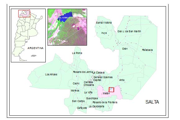
All of the above requires a combination of tangible and intangible aspects in a valid scale for decision-making, according to a new rationality (Saaty, 1996cited in Moreno Jiménez et al., 2001, p.6). (esm) on Environmental Impact Studies (eis) Within the general framework of the EIS, the Environmental Sensitivity analysis (ES) is incorporated in the Effects Prevention Stage, hand in hand, as the prospective process, with the members of the working group for further evaluation of EI. Moreover, the ESM are instrumental simulation models (Moldes, 1995) itself, which can be the base for a preliminary assessment of the current conditions of the environment against the actions foreseen in the project's idea stage. ESM also represent an input to perform reports on Environmental Impact Statement (EIS), as required by the relevant public authorities for smaller projects. A case study is presented for the implementation of an ESM for the construction and operation of a aqueduct for the provision of water for an ammonium nitrate production plant, located nearby the town El Tunal, Metán Department, Salta Province, Argentina (Figure 2). Four alternatives were analyzed for mentioned aqueduct traces, depending on the environment sensitivity.
2. II. Environmental Sensitivity Maps
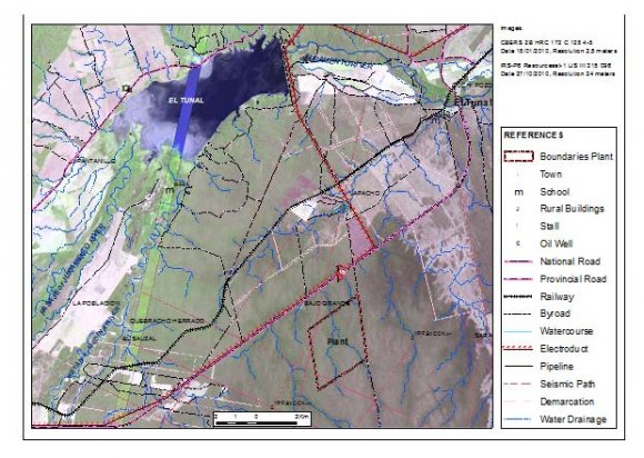
The area under analysis is presented in Figure 3, showing the site where the ammonium nitrate production plant will be installed, which requires a permanent water supply.
3. Methodology
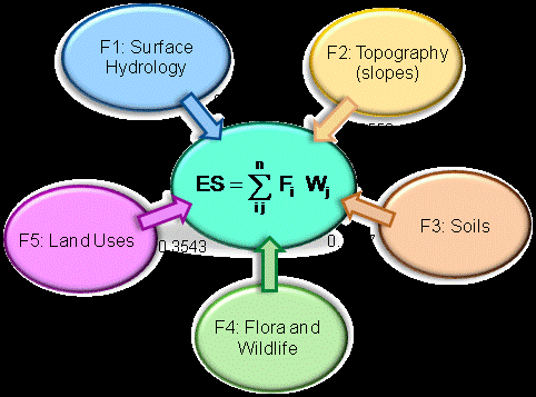
For Environmental Sensitivity analysis an index has been designed, in which three components of Environmental System Matrix Importance (physical, biological and socioeconomic) were considerate.
To evaluate Physical Environment sensitivity, these factors were established: hidrology -surface runoff (lotic) and surface water (lentic) -, topographythrough the slope -and finally, soils (Soil Groups and Suitability Classes).
To construct the factor for Biological Environment a combination of conservation value index, obtained for plant communities and birds, was used.
The Social-economic Environment was assessed in terms of the different land uses in the area and its related infrastructure, reflecting also on the degree of involvement that economic activities may suffer.
Factors (criteria) were selected by specialists from an initial hierarchical list, according to the relevance defined for the project objectives.
Environmental Sensitivity map (Figure 16) was obtained by the weighted sum of the sensitivity maps for each factor, as shown in Figure 4. Maps of sensitivity for each factor were standardized on a scale of 0 -10, 10 being the maximum value. Analytical Hierarchy Process copes with using original data, experience and intuition in the same model in a logical and through way (Forman, 1999
cited in Büyükyazici, Sucu, 2003).Then, a set of weights for each of the factors was established. The analyst worked in group with specialists to complete the comparison matrix in pairs. Wondered to each specialist individually to estimate a rating and the group if it was agreed to start the debate. The consensus was not difficult to achieve with this procedure.
4. a) Factor 1 -Surface Hydrology
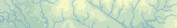
The drainage network was derived from a Digital Terrain Modeling (ASTER satellite, resolutions 30 m -Figure 5) and interpreted from high spatial resolution images (CBERS 2B HRC, resolutions 2.5 m Figure 3).
Comparisons are made in pairs and concern the relative importance of the two criteria involved in determining suitability for the stated objective. Ratings are provided on a nine-point continuous scale (Eastman et al., op. cit.). The equation was developed to mitigate the sensitivity to drainage networks environment and to achieve a gradual reduction in sensitivity as a function of distance from the axis of each drainage (talweg). The exponent allows to adjust the spatial scope of sensitivity according to the importance of the hydrology factor in the environmental context (Figure 5). The environmental sensitivity for the physical environment, was directly related to the environmental susceptibility to erosion, capable of generating economic or social involvement and in whose prediction, prevention or correction geomorphologic criteria should be used. For the orderly classification of slopes an exponential function was used y = 0.1749 e 0.6409x. Then S factor (steepness: Revised Universal Soil Loss Equation -RUSLE -) was calculated (Foster et al., 2003). Finally, the following linear equation was used: y = 0.882x + 0.745, with an R2 = 0.942, for assigning values of topography sensitivity by the S factor.
5. c) Factor 3 -Soils
Considering the characteristics of Soil Associations (Nadir and Chafatinos, 1995) present in the area under analysis the Soils Sensitivity map was generated (Figure 13). In this case, the Soils Group, the Suitability Class and the type of landform that corresponds to each unit were considerate (Table 3).
6. ( B )
7. d) Factor 4 -Flora and Wildlife
Considering both, the importance and the conservation status of different flora and wildliferepresented mainly by birds as indicators of environmental condition-, the fourth factor was built (Table 4). A good environmental quality has a greater number of animal populations.
8. ( B )
Table 4 : Values assigned to the categories of factor 3: Sensitivity for Flora and Wildlife Units.
9. Flora and
10. f) Alternatives Trace
As it has already been said, four alternatives of the aqueduct trace were compared, such alternatives are analyzed according to environmental sensitivity of the areas traversed. The alternative path was defined by the engineers in charge of the hydraulic aspects project, taking into consideration the possible water taking sites (Figure 10).
11. ( B )
e) Factor 5 -Land Use Considering Land Use, the fifth sensitivity factor was created that includes the categories listed and valuated in Table 5. As part of alternatives analysis, the optimal path algorithm (PATHWAY: IDRISI Taiga V. 16.05) was applied, using the Environmental Sensitivity map as friction (Figure 16).
IV.
12. Results
Below are the sensitivity maps obtained for each factor. For Environmental Sensitivity analysis a sample at random points 100 was extracted, probability distribution is shown in Figure 17, while the descriptive statistics are presented in Table 6.
13. Frecuency
14. Class
15. Environmental Sensitivity
The average of environmental sensitivity is within the interval ± 0.22 respect to the average of the sample with a probability of 95%.
16. a) Alternatives Trace Analysis
All alternatives trace run through areas with medium to low environmentally sensitivity. The greater environmental sensitivity is present in the trace for Alternative 3, followed by 4, then 2 and finally 1. It should be taken into account that: Alternatives 1, 2 and 4 have values close to environmental sensitivity and did not differ between them in more than 23.7%. (Table 7 and Figure 18). To the traces defined by Optimal Path, Environmental Sensitivity decreases for all alternatives, although that increases the length of the trace 3p and 4p. (Table 7 and Table 8). Comparing the alternatives 1 and 1p, the second reduced 29% environmental sensitivity respect to the first. Finally we conclude that the trace 1 and 1p presents the lowest environmental sensitivity. Managers must be decide what is the final trace, taking into consideration other criteria such as the costs of construction and operation.
V.
17. Discussion
Environmental Sensitivity is a concept closely linked to landscape as a complex system. Quantifying the landscape through indexes, reduces system complexity allowing spatial pattern analysis, and process alterations under study.
Environmental Sensitivity Maps are an instrumental model that provides adequate and sufficient information for understanding current conditions and the ability of the landscape to absorb new actions.
Environmental Sensitivity analysis can be incorporated into the forecast stage of Effects on Environmental Impact Studies. Environmental Sensitivity Maps represent an input for carrying reports on Environmental Impact Statement.
Hydrological Sensitivity equation allowed to integrate spatially the hydrologic factor as a decreasing continuous variable from drainage networks and water bodies. This function solves the problem of localized effect of the valuation of discrete entities.
Environmental Sensitivity Maps showed consistency in the analysis of alternatives for the location of new infrastructure. The combined use of environmental sensitivity map and the Pathway method allowed to define alternatives of trace for the aqueduct more efficiently from environment perspective.
VI.


| Topographic sensitivity (slope). | |||
| Class | Slope (%) | S Factor RUSLE | Sensitivity |
| 1 | 0.0 -0.3 % | 0.06 | 0.01 |
| 2 | 0.3 -0.6 % | 0.09 | 0.08 |
| 3 | 0.6 -1.2 % | 0.16 | 0.27 |
| 4 | 1.2 -3.0 % | 0.35 | 0.64 |
| 5 | 3.0 -6.0 % | 0.68 | 1.25 |
| 6 | 6.0 -9.0 % | 1.01 | 2.16 |
| 7 | 9.0 -12.0 % 1.50 | 3.43 | |
| 8 | 12.0 -25.0 % 3.57 | 5.12 | |
| 9 | 25.0 -50.0 % 7.01 | 7.29 | |
| 10 | > 50.0 % | 11.38 | 10.00 |
| Code | Soils Associations | Soils Group | Sensitivity |
| Ao-Lpb | Arrocera -La Población | C | 3.92 |
| Cho | Chorroarín | C | 3.92 |
| Lvi | Las Víboras | E | 1.68 |
| Oll-Etu | Olleros -El Tunal | B-C | 5.28 |
| Sig | San Ignacio | B | 7.22 |
| Sma | Santa María | C | 3.92 |
| Ts-Sun | Tuscal -Sunchal | C | 3.92 |
| Land Use | Sensitivity |
| Average | 3.36037583 |
| Standard error | 0.11033639 |
| Median | 3.44382751 |
| Mode | 1.46900749 |
| Standard Deviation | 1.10336387 |
| Sample variance | 1.21741184 |
| Kurtosis | -0.41780406 |
| Asymmetry coefficient | 0.17337022 |
| Rank | 4.21480226 |
| Minimum | 1.37450743 |
| Maximum | 5.58930969 |
| Sum | 336.037583 |
| Account | 100 |
| Confidence level (95.0%) | 0.21893137 |
| Environmental |
| Sensitivity |