1. Introduction
here has been a growing concern from scientific communities across the globe on analyzing spatiotemporal dynamics of rainfall and temperatures. As these two critical weather elements exerts overriding influence on agriculture and other aspects of human society, triggered by the increase in anthropogenic greenhouse gas emission causing the warming of the globe (IPCC, 2007). The global warming phenomenon creates series of feedback mechanisms affecting the natural processes of the hydrologic cycles which alters rainfall patterns in terms of intensity, duration, frequency, and onset and cessation. Although the issue of climate change has become a global issue, yet its impacts are rather deterministic in nature and depends on the specific region of concern (Amirabadizadeh , Huang, & Shui Lee, 2015). Global temperature studies have clearly reported on the recent long-term warming of the global around the middle of 1970 to 2013 with an average global trend of 0.2 ºC per decade (Rohde et al., 2013;Turco, Palazzi, Hardenberg, & Provenzale, 2015).
Though, in recent times the global temperature trends all over the world have either declined or lacks statistical significance in a lot of regional series around the globe around 1997 (Kaufmann, Kauppi, Mann, & Stock, 2011), although temperatures have consistently hovers above the long-term averages (Campra & Morales 2016). Recent observations and global averages show a significant decrease in the warming trend from 0.12 °C per decades between 1951-2012 to 0.05 °C per decades between 1998 to 2012 (Hartmann et al., 2013). Moreover, surface air temperatures exhibits greater spatial and temporal variability (Lovejoy, 2014;Steinman, Mann, & Miller, 2015;Turco et al., 2015).
Previous studies conducted to analyse the trends in the temperature and rainfall used Mann -Kendall statistics and Theil Sen's slope mainly due to the simplicity and versatility of the approach (Mustapha, 2013). For instance studies in India, by Jain and Kumar (2012) studied trends in rainfall, rainy days and temperature over India using Sen's non-parametric estimator and Mann-Kendall test. Their findings showed inconsistent rainfall trends amongst the stations under their study, 15 basins indicated decreasing trend with only one station showing statistically significant trend at 95% confidence level, while the mean maximum temperature series showed a rising trend for most of the stations; it showed a falling trend at some stations. The mean minimum temperature showed a rising as well as a falling trend. Also in the north-eastern United States, (Karmeshu, 2012) similarly used Mann-Kendall test on annual temperature and precipitation for the nine states, their findings revealed statistically significant increasing trend in temperatures for seven out of the nine states with annual linear trend ranging from 0.0006 to 0.02 o F per annum.
In a more recent studies, Chakraborty et al. (2017) studied changes in mean air temperature in the parts of eastern Himalaya, in the northeast Indian states. They observed spatial variability in trends with statistically significant increase in annual mean temperature for most of their stations. Despite the spatial variability, the overall range of increase in mean temperature is 0.2 °C to 1.6 °C per decade across the study region. Significant rise in average temperature during the winter is experienced by five out of seven places. While in Austria Herath and Sarukkalige (2017) using binning technique have reported variation of rainfall-temperature scaling with location and reported increasing trend for more extreme short span precipitation and a decreasing trend in the average long span precipitation incidences. The Fifth Assessment Report (AR5) of the intergovernmental panel on climate change (IPCC) revealed that the period 2016 to 2035 will witness increase in the mean temperature around the globe (Stocker et al., 2013). As such the need for the determination of local as well sub-regional trends and variability for a better understanding of the pattern of changes in the world climate has been reiterated (Campra & Morales 2016).
In spite of this growing concern and the prevalence of the trends associated with a number of climatic variables all over the world, studies of this nature in Malaysia are limited in number (Amirabadizadeh et al., 2015). A study by Wai, Camerlengo, Khairi, and Wahab (2005) reported an upward trend in the average yearly temperature. Their studies predicted temperature changes ranging from 0.99 o C to 3.44 o C for the next one hundred years. They also reported upward warming trend for all their stations for the past three decades. Tangang, Juneng, and Ahmad (2007), also reported a warming trend of 2.7 -4.0 o C per 100 years for all regions in Peninsular Malaysia and the northern Borneo. Studies by (Suhaila, Deni, Zin, & Jemain, 2010; Varikoden, Preethi, Samah, & Babu, 2011; Zin, Jamaludin, Deni, & Jemain, 2010) have equally demonstrated the variability and occurrence of extreme events signalling changes in the pattern of climate in some parts of the country with its attendant consequences on the environment and other activities.
Similarly, the study by Amirabadizadeh et al. (2015) reported a warming trend of minimum and maximum temperatures ranging from 3.5 o C to 4.0 o C per 100 years (0.035 o C to 0.04 o C per annum) over the Langat River Basin in Malaysia. Suhaila and Yusop (2017) used Pettit and sequential Mann-Kendall (SQ-MK) tests to examine the annual and seasonal trends, and change point detection associated with the mean, maximum and minimum temperature data series in Peninsular Malaysia. Their findings detected abrupt changes in the data series and observed significant increasing trends in the annual and seasonal mean, maximum and minimum temperatures in over the country ranging from 2 to 5 °C per 100 years during the last 32 years. They detected large increase in magnitudes of the minimum temperature trend greater than that of the maximum temperatures for most the stations under study.
A number of possible factors governing spatial and temporal variability of surface temperature warming in a particular region or continental area have been highlighted in the literature. They include those related variability arising from atmosphere-ocean interface. For example North Atlantic Oscillation (NAO), the Pacific Decadal Oscillation (PDO), the Indian Ocean Dipole (IOD) and the El Ni-no-Southern Oscillation (ENSO).
The variability of inter-annual temperatures perhaps have largely been ascribed to the effects of El Ni-no -Southern Oscillation (ENSO) and El-Nina (Suhaila and Yusop (2017). In parts of Southeast Asia recent study by Malik et al. (2012) visualized the pattern of extreme events in the rainfall-fields revealed the variability in the moisture sinks over the region. These natural variabilities are believed to have caused both inter-annual and decadal variations of temperatures in some part of the globe and may influence the long term warming trend in any part of the world (Tangang et al., 2007), as well rainfall variability (Tan, Ibrahim, Cracknell, & Yusop, 2017).
Beside these, other anthropogenic ally induced variability, such as the consequences of the Urban Heat Island (UHI) (Li, Zhang, Liu, & Huang, 2004; Philandras, Metaxas, & Nastos, 1999), and deforestation effects (Voldoire & Royer, 2004) are capable of causing variation in the local patterns of temperatures. But in the case of Malaysia and perhaps major part of Southeast Asian sub-region studies have demonstrated continuous changes in the inter-annual rainfall variability and other anomalies (Juneng & Tangang, 2005;Tangang et al., 2007). Furthermore, Tangang et al. (2007) averred that Malaysia being located amid the Indian and the Pacific Ocean which is the origin of the expanding Walker cell, it is probable that the IOD might have an effect on the country's temperature and rainfall variation. Hence the need for more studies on the rainfall behaviour especially at the micro levels to effectively comprehend the significance of the climatic changes has also been stressed (Suhaila et al., 2010).
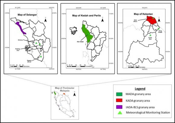
This study analyzed and examined the trend in the changes associated with minimum and maximum annual, monthly and seasonal scale temperatures specific to the granary areas of MADA, Kedah, IADA, Barat Laut Selangor, and KADA, Kelantan in the Peninsular Malaysia. The study however employed Theil-Sen's Slope and measured the rate of changes of these variables temporally.
2. II.
3. Materials and Methods
4. a) Data Sources
Time series data for mean monthly values of temperature for the period of Generally, the need to identify outliers is one of the significant step in the data quality control (González-Rouco, Jiménez, Quesada, & Valero, 2001). Outliers could be error in measurement or might be accurate extreme values. In the context of this dataset, the concern was not identification of erroneous observations especially with the regards to using hydrological parameters, but to reduce the size of the distribution tails (González-Rouco et al., 2001). In this study, possible outliers were examined using Q-Q plots of the individual data sets, the identified possible outliers were corrected by trimming the extreme values relative to the mean value. In this case outliers were considered as those values above a maximum threshold for each of the time series (González-Rouco et al
5. d) Homogeneity Test
In this study the test of inhomogeneity of datasets (temperature series) was performed by applying four techniques of the standard normal homogeneity test, Buishand range test, Pettitt test, and Von Neumann ratio tests. The results showed that the data series obtained from the three stations were found to be homogeneous at ? = 0.05.
6. e) Linear Regression Test
Simple linear regression is considered as a conventional approach and one of the simplest methods used in detecting changes in the time series of meteorological variables (Campra & Morales 2016). Simple linear regression was applied to the temperature and rainfall data series. Trends and their 95% CIs were estimated by least squares linear regression. Linear trends were estimated in every series from the slopes of the fit using values of monthly, annual and seasonal averages of Tmax, Tmin ( Where X 's are the K explanatory variables (years) and y is the dependent variable (maximum temperature, minimum temperature). The slope line is b, and a is the intercept (value of y when x =0). The slope of regression describes the trend whether positive or negative. Linear regression works with the assumption of normal distribution. In this instance, the null hypothesis is that the slope of the line is zero or there is no trend in the temperature data. The significance of the slope shows the probability value (p-value). Microsoft excel was therefore, employed in the plotting of the trend lines and the Xlstat was used in the determination of the statistical values of the linear regression analysis. The P-value from the regression analysis was tested at the significance level ? = 0.05. The R 2 value or the square of the correlation from regression is used to indicate the strength of association and relationship between the variables X and Y. It has ratio between 0 and 1.0. R 2 value of 1.0 indicates stronger correlation and it means all points lie linearly. Whereas when R 2 is 0.0 it means no correlation or linear relation between variables X and Y.
7. f) Mann Kendall Trend Test
In this study Mann Kendall test was used to examine the performance of a class of non -parametric trend test and the relative magnitude of the data rather than their measured values (Juahir et al., 2010;Kendall 1975). In this context the method was used to detect long term trend of the meteorological variables (i.e. temperature) in the respective study areas.
Monthly and annual series were determined for each of the station using the seasonal Mann Kendall Trend Test (Juahir et al., 2010;Río et al., 2011). XLSTAT software was used in the graphical presentation of the data sets. Moreover, XLSTAT and MAKESEN software were also used to calculate the statistical significance and estimation of trend using Sen Slope estimator for the variability and trend detection (Río et al., 2011).
The underlying principle of this model was based on the statistic (S) which is considered to be zero (0) meaning there was no trend. Each pair of observed values y i, y j (1> j) of the random variable was examined to find out whether y i > y j or y i < y j . The test statistic for the Mann-Kendall test was given as;
S = ? ? ?????? ??? ?? ? ?? ?? ? ?? ?? =?? =1 ???1 ???1 (2.3) Where; Sign??? ?? ? ?? ?? ? = ? 1 ???? ?? ?? ? ?? ?? = 0 0 ?????? ?? ? ?? ?? = 0 ?1 ?????? ?? ? ?? ?? = 0 ? (2.4)This means that the number of positive differences minus the number of negative differences. Variance of s is therefore computed by;
Var (s) =[??(?? ? 1)(2?? + 5) ? ? (?? ? 1) ?? (2?? + 5)]/18 (2.5)In a situation where n is greater than 10, the standard normal variate z is computed by using the following equation (Douglas, Vogel, & Kroll, 2000).
Z = ? ? ? ? ? ???1 ??????? (??) ???? ?? > 0 0 ???? ?? = 0 ??+1 ??????? (??) ???? ?? < 0 ? ? ? ? ? (2.6)Therefore, the presence of a statistical trend is assessed using z value. A positive or negative z value is an indication of upward or downward trend. This study used Sen Slope estimator which is a non-parametric test procedure discovered by Sen (Sen 1968) and advanced by (Gilbert, 1987) to measure the actual slope in Mann -Kendall trend tests. It estimates the degree of any significant monotonic increase or decrease in trends examined in the Mann -Kendall S tests. The estimator Sen Slope was used where trend identified in the time series data is considered to be linear, illustrating the measure of the change per unit time (Mustapha, 2013;Tabari & Talaee, 2011). The Sen Slope estimator method is not sensitive to single data error or outliers. It is represented in the following equation;
Q = ???? ?? ? ???? ?? (2.7)Where Q represents the value of Sen in slope estimator; xj and xk are data values at time j and k. If there are n values of xj in the time series, the Sen Slope estimator is the median of n(n-1)/2 pairwise slopes, hence the Sen Slope estimator can be determined using;
Q = ??? ??+1 2 ????? ?????? ?????? (2.8) Q = 1 2 (?? 2 ?? ) + ??? ??+2 2 ? ???? ?? ???? ???????? (2.9)III.
8. Results & Discussions a) Descriptive Statistical Analysis
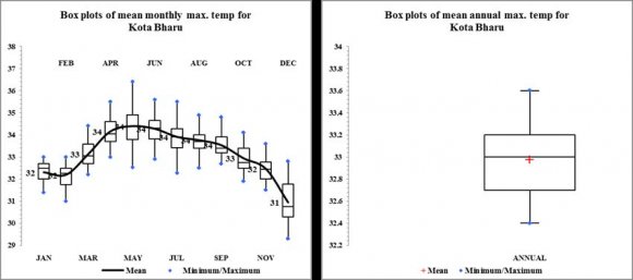
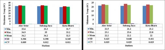
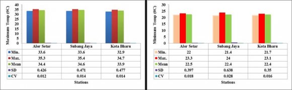
Table 1 provides a simple descriptive statistics of the annual values for the three variables used in this From the mean temperature records (Table 1), it is evident that Subang Jaya station recorded the highest mean maximum temperature of 34.5 o C, followed by Alor Setar (34.4 o C) and Kota Bharu station observed the lowest mean maximum temperature (32.9 o C). For the Mean minimum temperature values, Subang Jaya observed the highest mean followed by Alor Setar and Kota Bharu recorded the lowest mean. Alor Setar and Subang Jaya observed average maximum temperature slightly higher than the Malaysia average (33 o C), while Kota Bharu station exhibited average maximum temperature almost the same with that of Malaysia. Similarly, all the three stations observed slightly higher average minimum temperature than the mean minimum temperature value of 22.0 o C for Malaysia (Chee-Wan & Meng-Chang, 2012).
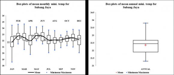
The values of the standard deviation further revealed the absolute variability of the temperatures. Subang Jaya station observed the highest absolute variability as indicated by the coefficients of standard deviation of 0.45 and 0.66 for both minimum and maximum temperatures respectively. Alor Setar recorded second highest standard deviation of 0.39 for the maximum temperature. Kota Bharu station observed the lowest standard deviation of 0.32 for the maximum temperature, but observed higher standard deviation of minimum temperature next to Subang Jaya. The coefficient of variability (CV) relatively indicated that Subang Jaya had the highest coefficient of variation of 0.013 in annual maximum temperature, Alor Setar observed second highest coefficient of variability (0.011) for maximum temperature. While Subang Jaya and Kota Bharu observed highest minimum temperature coefficient of variation of 0.029 each.
Table 2 indicates the pattern of the temperature variability when the temperature variables were constructed into 10 year intervals to examine their possible changes in the mean, standard deviation and the coefficient of variability over time. In Alor Setar station the changes in mean annual maximum temperature and the mean annual minimum temperature were first steady, and between the periods 2001 to 2010 the mean annual maximum temperature and the mean annual minimum temperature appreciated with about 1.5% and 0.9% respectively with the decreasing variability.
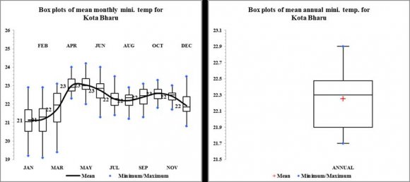
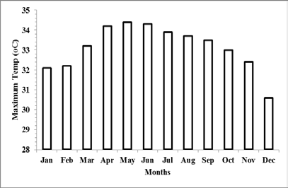
For the Subang Jaya station, the mean annual maximum temperature decreased with about 6% within the 30 years period, while the mean annual minimum temperature increased by about 2.8% within the periods, but there were general increased in the temperature variability. At Kota Bharu station both the mean annual maximum and mean annual minimum temperatures increased by 0.3% and 2.8% respectively, with 1.1% relative variability. The highest mean monthly minimum temperature also coincided with the month of February (Figure 4). In Kota Bharu station (Figure 6), there is little variation in the mean monthly maximum temperature throughout the year, yet the month of May was the warmest (34.4 o C) followed by the month of June (34.3 o C) and the lowest mean maximum temperature corresponded with the month of December (30.6 o C). Also, average minimum temperature in this station indicates little variability (Figure 6). Characteristically the average minimum values peaked correspondingly along with the months of higher average monthly maximum temperature, which is April with 23 o C; but, the months of January through February were noted to be less warm (Figure 7). For the purpose of this study, the seasonal variability in terms of temperature were analysed based on the two paddy growing seasons, i.e. the main season is considered as the period when paddy is grown without supply of water from irrigation . Though varies usually from August/September to February/Mach the following year. The off season is regarded as the dry period when paddy planting normally depends on an irrigation system, the time mostly span from February/March until July/August (DOA, 2014). In this respect, Figures 7-8 presents the descriptive statistics of the seasonal temperatures for the period 1981 to 3014 in the study areas.
From Figure 8 the mean temperature for the main season was generally lower than the off season temperatures, probably due to the moderating effect of the relatively high amount of rainfall received during the main season. Comparatively, MADA and IADA recorded high mean maximum temperature of 34.2 o C each, while KADA had the lowest mean maximum value (32.3 o C).
During the off season (Figure 9),Subang Jaya station representing IADA recorded the highest mean maximum temperature (34.6 o C) followed by Alor Setar representing MADA (34.4 o C) and Kota Bharu station representing KADA also had the lowest mean. There was higher maximum temperature variability in IADA during the main season, in the MADA area showing less variability (Figure 8). But, in Figure 9, during the off-season the maximum temperature is more variable at IADA and KADA than at MADA. The minimum temperature shows greater variability more than the maximum temperature for all the seasons in the three areas. Comparatively, the main season minimum temperature for IADA is more variable than in MADA and KADA (Figure 9). But, minimum temperature for KADA was the least variable during the off-season compared to MADA and the highest variability of minimum temperature was observed in IADA during this season (Figure 9).
9. b) Ordinary Linear Regression Trend Analysis
The result of the linear regression of the annual, monthly and seasonal maximum temperature, minimum temperature and rainfall trend analysis for the three study areas are calculated for the34 years independently.
10. c) Maximum Temperature Regression Analysis
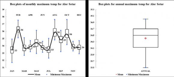
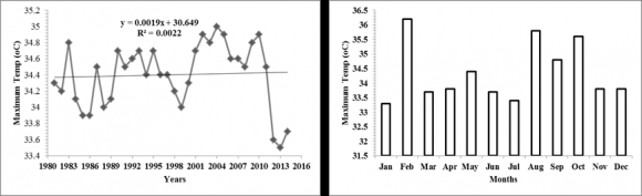
The maximum temperature linear regression analysis for Alor Setar was conducted on the annual and monthly values, in Alor Setar, the linear trend line of the annual mean maximum temperature shows increasing trend, although there was a weak relationship between the maximum temperature changes and year (R 2 = .002) as illustrated in Figure 10a. Higher mean maximum temp is recorded in the months of February, August and October (Figure 10b). As for the monthly maximum temperature trend, the months of March, April, May, July and November showed decreasing trend, but the other months demonstrated an increasing trend. From the probability value (p-value) of the regression analyses, the coefficients of the monthly and annual trend lines were greater than 95% confidence level (?=0.05), the null hypothesis (that there is no significant trend in the annual and monthly maximum temperature is therefore retained). This means that the annual and monthly maximum temperature exhibited no statistically significant trend, except for the months of January and February. The regression result also shows that more warming was recorded in the month of February with coefficient of .045 0 C with a unit change in the year.
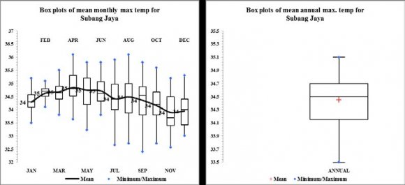
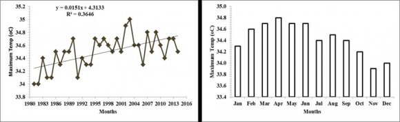
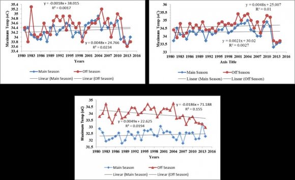
Figure 11a shows the annual maximum temperature increasing linear trend with a moderate relationship between maximum temperature changes and the year (R 2 = .365), while Figure 11b illustrates the monthly maximum temperature pattern for Subang Jaya over the years. The maximum temperature linear regression analysis was further conducted on the annual and monthly values. The result showed that both annual and monthly maximum temperature demonstrated increasing trend. Only the months of January, February and March revealed statistically significant upward trend. There was no statistically significant increasing trend for the rest of months at 95% confidence level. The maximum temperature for the month of March revealed more significant warming trend with the coefficient of .046 0 C for every unit increase in the year (p = 0.000). Figure 13 shows the seasonal mean maximum temperature trends for the three study areas. The off seasons maximum temperature for Alor Setar and Kota Bharu showed decreasing trend, while the maximum temperature for all the seasons in Subang Jaya and main season in Alor Star and Kota Bharu showed increasing trend. All the R 2 shows a weak relationship between seasonal maximum temperature changes and the changes in the year.
The result for the linear regression indicated that only main season maximum temperature at Subang Jaya representing IADA showed statistically significant upward trend for the period with a coefficient of .016 (p = .002). Also the off seasons, mean maximum temperatures for Alor Setar representing MADA and Kota Bharu representing KADA revealed statistically significant downward trend with the coefficient of -.031 (p = .004)and -.022( p= .033) respectively.
11. ) Minimum Temperature Regression Analysis
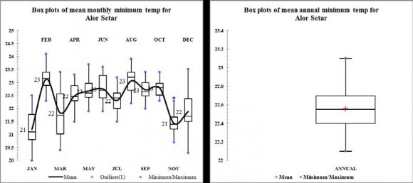
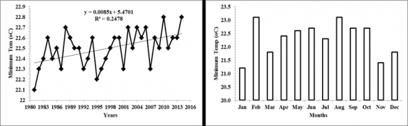
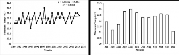
Figure 14a shows the linear trend of the annual minimum temperatures while Figure 14b shows the mean monthly minimum temperature pattern. The result from the regression analysis on the mean annual minimum temperature and mean monthly minimum temperature for Alor Setar showed increasing trends for all the months as well as the mean annual minimum temperature. But only the minimum temperature for the months of February and July were shown to have no statistically significant trend at 95% confidence level (? = .050). From the coefficients of the regression analyses, the minimum temperature for the month of March recorded highest increasing trend within the period with the coefficient of .054 0 C (p =.000). The lowest increasing trend was recorded in the month of
12. Kota Bharu
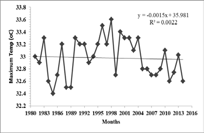
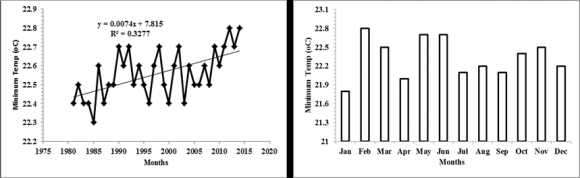
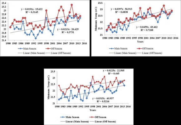
Subang Jaya Alor Setar October with coefficient of .014 0 C (p =.000). The monthly increasing minimum temperature trend for the month of March surpasses the annual increasing trend over the years with coefficient of .018 0 C (p = .000). R 2 shows a weak relationship between annual minimum temperature changes and the year. 15 a shows the annual linear trend for the mean minimum temperature for Subang Jaya with moderate relationship between annual minimum temperature changes and the year (R 2 = .328), while Figure 15b shows the pattern of the mean monthly temperatures. From the linear regression analysis, the result shows statistically significant upward trend for all the monthly and annual mean monthly minimum temperature for this station. The linear trend coefficient for the mean monthly minimum temperature ranges from .037 0 C to .063 0 C. The highest increasing trend was recorded in the month of March, while the months of June and July were the lowest increasing trend. Figure 17 shows linear trends of seasonal mean minimum temperature trends for both main and off seasons for the three stations. The regression result for the seasonal changes in the mean minimum temperatures (Appendix F) showed statistically significant increasing trends for all the seasons. Subang Jaya recorded higher upward trend for all the season with the coefficient of .058 (p =.000) each. Alor Setar recorded lowest trend during the main season, while during the off-season Kota Bharu station recorded the lowest seasonal minimum temperature trend. All the R 2 values show that substantial changes in the seasonal temperatures were determined by the changes in the time (year). In Table 3 present the results of Mann-Kendall and Sen's slope estimator for the mean annual and mean monthly maximum temperatures for Alor Setar. Based on this result the maximum annual temperature indicated a statistically not significant increasing trend in the data series. The MK test confirmed the result of the regression analysis which shows no statistically significant increase in the annual maximum temperature. Mann-Kendall trend revealed similar pattern of upward and downward trends. Similar to the linear regression analysis, the months of March, April and November have negative sign signifying decreasing trend in the monthly maximum temperature. While the months of May, July and October indicated no trend in their monthly maximum temperature, the rest of the months showed positive sign indicating increasing trend. From the result only the mean maximum temperature for the months of January, August and September shows statistically significant increasing trend. Highest warming was indicated during the months of January (Z= 2.69; Q = 0.05). Table 4 presents the result from the Mann-Kendall and Sen's slope estimator for the annual and monthly maximum temperature for Subang Jaya station. All the monthly and annual maximum temperature for this station revealed increasing trend with the exception of the months of October and November exhibiting no trend and decreasing trend in the maximum temperature respectively. Only the months of February, March, April, September, and the annual maximum temperature for this station revealed statistical significant increasing trends. The MK trend test result confirmed the regression analysis where both the two tests revealed increasing trends in all the monthly maximum temperature except for the October maximum temperature. Table 5 shows the result of the Mann-Kendall trend test and Sen's slope estimator for the annual and monthly maximum temperature for Kota Bharu station. The result shows a downward trend in the months of January, February, September and November maximum temperature, while the maximum temperature for the month of June showed no trend. All other months including the annual maximum temperature showed increasing trend. There were no statistically significant trends for all the months except for July, December and the annual maximum temperature at 95% confidence level (? =.05). Table 6 presents the result of Mann-Kendall trend test and Sen's slope estimator for the seasonal maximum temperature for the three stations. The result shows increasing trend in the maximum temperature for all the seasons in all the three study areas. Moreover, only the off-season temperature in all the three areas showed statistically significant increasing trend. More warming is observed during the off-season in Alor Setar (Z= 2.38; Q= .032) higher than all the other areas. The MK test result is similar to the regression analysis for seasonal maximum temperatures. 7 revealed statistically significant upward trends in minimum temperature records for all the months as well as for the annual values over the periods in Alor Setar, except for the months of February and July. The rising minimum temperature was observed to be significantly higher in the month of March (Z =3.73; Q = 0.056), whereas lowest significant increasing trend in the monthly minimum temperature was noticed in the month of October (Z= 2.15; Q=.0014). The MK trend statistics confirmed the regression result of the minimum temperature for this station. Table 8 shows the result of Mann-Kendall and Sen's slope estimator for the minimum temperature in Subang Jaya stations over the years. The result revealed statistically significant increase in the minimum temperature for all the months as well as the annual minimum temperatures with the exception of the month of July which showed no trend at 95% confidence level. Statistically significant upward warming corresponded with the month of March, December and the annual value with (.063 o C) each. The month of August recorded the lowest significant minimum temperature warming (.0.028 o C). The result confirmed the regression result for the minimum temperature for this station. Table 9 shows the result of Mann-Kendall tests and Sen's slope estimator for monthly and the annual minimum temperature of Kota Bharu station. The result revealed increasing trend in the monthly as well the annual minimum temperature over the periods. But, the minimum temperature for the months of May and November were statistically not significant, while all the rest of the months as well as the annual values showed statistical significant increasing trends at 95% confidence level.
For all the monthly temperatures, January minimum temperature observed the highest upward trends (Z= 3.21; Q= .056), while the month of April recorded the lowest upward trend (Z = 2.15; Q= .018). The result of Mann-Kendall and Sen's slope estimator of seasonal minimum temperature for the three stations are presented in Table 10. The result revealed statistically significant increasing trend for the minimum temperature in all the seasons. The rising seasonal minimum temperature was higher for all the seasons in Subang Jaya station, while Kota Bharu station observed the lowest upward trend for the two seasons.
13. Summary
In summary, the variability of temperature in the three study areas were investigated using descriptive statistics, parametric (least square regression) and nonparametric (Mann-Kendall and Sen's slope estimator). The study identified significant warming trend in the annual mean maximum temperature in two of the study areas, i.e. Subang Jaya and Kota Bharu typifying the climate over Peninsular Malaysia. Also significant warming trend detect in the annual minimum temperature and significant increasing trend in some of the monthly maximum and minimum temperatures for all the three stations. Also, the result reveals spatial and temporal variation in both the maximum and minimum temperature at annual, monthly and seasonal scales.
For the annual scale maximum temperature, this study identified a warming trend for the two stations with about 0. V.
14. Conclusion
Firstly, it can be concluded that there were spatial as well as temporal variation of temperature across the three granary areas. Secondly, the study identified significant warming trend in the annual mean maximum temperature in two of the study areas, i.e. Subang Jaya and Kota Bharu. Also significant warming trend were detected in the annual and seasonal minimum temperature for all the stations as well as significant increasing trend in some of the monthly maximum and minimum temperatures for all the three stations.
The findings from this study have the following implications; firstly, the result from the trend analysis provides an insight to agricultural development agencies in these areas and paddy farmers themselves, to make pre-emptive measure in relation to climate change variability. Timely measures and institutional actions will surely assist in ameliorating the damages that may be caused by the climate variability. This is in view of the fact that 34 years temperatures and rainfall data do not suffices the denial of the occurrence of climate change variability.
Funding: This research did not receive any specific grant from funding agencies in the public, commercial, or notfor-profit sectors.
15. Conflict of Interests:
The authors wish to summarily declare that they have no conflict of interest concerning the publication of this paper.
| Granary | Variables | Min | Max | Mean | SD | CV |
| Alor Setar | Tmax ( 0 C) | 34.4 | 35.0 | 34.4 | 0.39 | 0.011 |
| Tmin( 0 C) | 22.2 | 23.2 | 22.5 | 0.25 | 0.011 | |
| R/Fall(mm) | 1575.2 | 2626.4 | 2016.7 | 249.3 | 0.123 | |
| Subang Jaya | Tmax ( 0 C) | 34.5 | 35.1 | 34.5 | 0.45 | 0.013 |
| Tmin( 0 C) | 22.3 | 23.8 | 22.4 | 0.66 | 0.029 | |
| R/Fall(mm) | 1944.8 | 3210.3 | 2551.8 | 328.3 | 0.017 | |
| Kota Bahru | Tmax ( 0 C) | 32.9 | 33.6 | 32.9 | 0.32 | 0.010 |
| Tmin( 0 C) | 22.1 | 24.2 | 22.3 | 0.65 | 0.029 | |
| R/Fall(mm) | 1540.5 | 3734.5 | 2576.5 | 595.8 | 0.231 | |
| Data source: Malaysia Meteorological Department | ||||||
| Period | 1981 -1990 | 1991 -2000 | 2001 -2010 | |||||||
| Station | Statistics | Tmax ( 0 C) | Tmin ( 0 C) | R/F (mm) | Tmax ( 0 C) | Tmin ( 0 C) | R/F (mm) | Tmax ( 0 C) | Tmin ( 0 C) | R/F (mm) |
| Lowest | 33.9 | 22.3 | 1615.3 | 33.9 | 22.2 | 1473.5 | 34.5 | 22.3 | 1928 | |
| Alor Setar | Highest Mean SD | 34.8 34.2 0.327 | 22.7 22.4 0.131 | 2469.5 1989.8 284.2 | 34.8 34.2 0.327 | 22.6 22.4 0.141 | 2183.9 1911.6 193.4 | 35.0 34.7 0.162 | 22.9 22.6 0.164 | 2573.5 2248.8 193.5 |
| CV | 0.010 | 0.006 | 0.143 | 0.010 | 0.006 | 0.101 | 0.005 | 0.007 | 0.086 | |
| Lowest | 34.0 | 21.3 | 1971.3 | 34.3 | 21.8 | 2419.0 | 34.1 | 22.2 | 2292.4 | |
| Subang Jaya | Highest Mean SD | 34.8 34.3 0.241 | 22.1 21.6 0.287 | 3331.4 2390.9 405.5 | 34.8 34.5 0.171 | 23.0 22.3 0.323 | 2811.5 2646.5 126.1 | 35.2 34.1 0.359 | 23.3 22.6 0.294 | 3455.2 2908.1 320.7 |
| CV | 0.07 | 0.013 | 0.170 | 0.005 | 0.014 | 0.048 | 0.010 | 0.013 | 0.110 | |
| Min | 32.4 | 21.7 | 1540.5 | 32.7 | 21.9 | 1689.0 | 32.7 | 22.0 | 1928.6 | |
| Kota Bharu | Max Mean SD | 33.3 32.8 0.342 | 22.2 21.8 0.147 | 2859.3 2240.6 469.9 | 33.6 33.1 0.273 | 22.9 22.3 0.329 | 3734.5 2886.2 671.2 | 33.3 32.9 0.231 | 22.8 22.4 0.238 | 3566.2 2547.1 494.0 |
| CV | 0.010 | 0.007 | 0.210 | 0.008 | 0.015 | 0.233 | 0.007 | 0.011 | 0.194 | |
| Data Source: Malaysia Meteorological Department | ||||||||||
| Alor Setar | Subang Jaya | |||||
| Kota Bharu | ||||||
| Month | n | Z-Value | Theil Sen's Slope (Q) | Trends | Kendall's Tau | P-Value |
| Jan | 34 | 2.69 | 0.05 | Increasing | 0.329 | 0.007 |
| Feb | 34 | 1.25 | 0.025 | No Trend | 0.155 | 0.211 |
| Mar | 34 | -1.13 | -0.014 | No Trend | -0.139 | 0.259 |
| April | 34 | -1.05 | -0.02 | No Trend | -0.130 | 0.291 |
| May | 34 | 0.03 | 0.0 | No trend | 0.005 | 0.976 |
| Jun | 34 | 0.78 | 0.005 | No Trend | 0.098 | 0.438 |
| Jul | 34 | 0.22 | 0.0 | No trend | 0.029 | 0.823 |
| Aug | 34 | 2.41 | 0.029 | Increasing | 0.297 | 0.016 |
| Sep | 34 | 2.12 | 0.033 | Increasing | 0.260 | 0.034 |
| Oct | 34 | 0.43 | 0.0 | No trend | 0.056 | 0.665 |
| Month | n | Z-Value | Theil Sen's Slope (Q) | Trends | Kendall's Tau | P-Value |
| Jan | 34 | 1.16 | 0.025 | No Trend | 0.198 | 0.108 |
| Feb | 34 | 3.27 | 0.033 | Increasing | 0.405 | 0.001 |
| Mar | 34 | 3.20 | 0.050 | Increasing | 0.392 | 0.001 |
| April | 34 | 2.08 | 0.029 | Increasing | 0.255 | 0.050 |
| May | 34 | 1.53 | 0.024 | No Trend | 0.190 | 0.125 |
| Jun | 34 | 1.30 | 0.014 | No Trend | 0.161 | 0.195 |
| Jul | 34 | 1.38 | 0.020 | No trend | 0.170 | 0.167 |
| Aug | 34 | 1.32 | 0.030 | No Trend | 0.162 | 0.186 |
| Sep | 34 | 2.44 | 0.050 | Increasing | 0.300 | 0.015 |
| Oct | 34 | 2.48 | 0.039 | Increasing | 0.304 | 0.013 |
| Nov | 34 | -0.85 | -0.009 | No Trend | -0.106 | 0.396 |
| Dec | 34 | 1.40 | 0.013 | No Trend | 0.173 | 0.162 |
| Annual | 34 | 2.18 | 0.014 | Increasing | 0.275 | 0.029 |
| Month | n | Z-Value | Theil Sen's Slope (Q) | Trends | Kendall's Tau | P-Value |
| Jan | 34 | -1.04 | -0.025 | No Trend | -0.129 | 0.298 |
| Feb | 34 | -1.86 | -0.03 | No Trend | -0.229 | 0.063 |
| Mar | 34 | 1.65 | 0.021 | No Trend | 0.203 | 0.099 |
| April | 34 | 1.81 | 0.025 | No Trend | 0.223 | 0.070 |
| May | 34 | 1.11 | 0.007 | No Trend | 0.139 | 0.268 |
| Jun | 34 | 0.30 | 0.0 | No trend | 0.038 | 0.766 |
| Jul | 34 | 2.34 | 0.028 | Increasing | 0.288 | 0.020 |
| Aug | 34 | 1.25 | 0.013 | No Trend | 0.155 | 0.211 |
| Sep | 34 | -1.01 | -0.009 | No Trend | -0.127 | 0.311 |
| Oct | 34 | 1.26 | 0.013 | No Trend | 0.156 | 0.206 |
| Nov | 34 | -1.41 | -0.016 | No Trend | -0.175 | 0.158 |
| Dec | 34 | 2.69 | 0.038 | Increasing | 0.331 | 0.007 |
| Annual | 34 | 2.16 | 0.014 | Increasing | 0.270 | 0.031 |
| Max. Temperature | n | Z-value | Theil Sen's Slope(Q) | Trends | Kendall's Tau | P-value |
| Alor Setar_MS | 34 | 1.36 | 0.008 | No Trend | 0.170 | 0.175 |
| Alor Setar_OS | 34 | 2.38 | 0.032 | Increasing | 0.294 | 0.017 |
| Kota Bharu_MS | 34 | 0.69 | 0.004 | No Trend | 0.087 | 0.492 |
| Kota Bharu_OS | 34 | 2.11 | 0.025 | Increasing | 0.259 | 0.035 |
| Subang Jaya_MS | 34 | 3.02 | 0.016 | Increasing | 0.377 | 0.003 |
| Subang Jaya_OS | 34 | 1.65 | 0.017 | No Trend | 0.206 | 0.098 |
| f) MK Test for Minimum Temperature | ||||||
| Table | ||||||
| Month | n | Z-Value | Theil Sen's Slope (Q) | Trends | Kendall's Tau | P-Value |
| Jan | 34 | 2.56 | 0.033 | Increasing | 0.313 | 0.011 |
| Feb | 34 | 1.31 | 0.013 | No Trend | 0.163 | 0.190 |
| Mar | 34 | 3.73 | 0.056 | Increasing | 0.455 | 0.000 |
| April | 34 | 3.36 | 0.027 | Increasing | 0.417 | 0.001 |
| May | 34 | 4.29 | 0.031 | Increasing | 0.532 | 0.000 |
| Jun | 34 | 2.13 | 0.022 | Increasing | 0.264 | 0.033 |
| Jul | 34 | 1.71 | 0.012 | No Trend | 0.214 | 0.088 |
| Aug | 34 | 2.67 | 0.022 | Increasing | 0.333 | 0.008 |
| Sep | 34 | 3.02 | 0.024 | Increasing | 0.377 | 0.003 |
| Oct | 34 | 2.15 | 0.014 | Increasing | 0.267 | 0.032 |
| Nov | 34 | 3.64 | 0.027 | Increasing | 0.453 | 0.000 |
| Dec | 34 | 3.44 | 0.042 | Increasing | 0.425 | 0.001 |
| Annual | 34 | 4.16 | 0.018 | Increasing | 0.524 | 0.000 |
| Month | n | Z-Value | Theil Sen's Slope (Q) | Trends | Kendall's Tau | P-Value |
| Jan | 34 | 3.49 | 0.052 | Increasing | 0.425 | 0.000 |
| Feb | 34 | 3.03 | 0.040 | Increasing | 0.375 | 0.002 |
| Mar | 34 | 4.75 | 0.063 | Increasing | 0.584 | 0.000 |
| April | 34 | 4.72 | 0.057 | Increasing | 0.577 | 0.000 |
| May | 34 | 4.32 | 0.047 | Increasing | 0.530 | 0.000 |
| Jun | 34 | 4.15 | 0.050 | Increasing | 0.510 | 0.000 |
| Jul | 34 | 2.75 | 0.041 | Increasing | 0.337 | 0.006 |
| Aug | 34 | 2.33 | 0.028 | Increasing | 0.288 | 0.020 |
| Sep | 34 | 3.54 | 0.033 | Increasing | 0.437 | 0.000 |
| Oct | 34 | 4.33 | 0.040 | Increasing | 0.532 | 0.000 |
| Nov | 34 | 4.90 | 0.062 | Increasing | 0.599 | 0.000 |
| Dec | 34 | 3.45 | 0.063 | Increasing | 0.422 | 0.001 |
| Annual | 34 | 6.13 | 0.063 | Increasing | 0.751 | 0.000 |
| Month | n | Z-Value Theil Sen's Slope (Q) | Trends | Kendall's Tau | P-Value | |
| Jan | 34 | 3.21 | 0.056 | Increasing | 0.390 | 0.001 |
| Feb | 34 | 2.87 | 0.050 | Increasing | 0.351 | 0.004 |
| Mar | 34 | 2.41 | 0.044 | Increasing | 0.295 | 0.016 |
| April | 34 | 2.15 | 0.018 | Increasing | 0.268 | 0.032 |
| May | 34 | 0.57 | 0.004 | No Trend | 0.072 | 0.571 |
| Jun | 34 | 2.20 | 0.023 | Increasing | 0.272 | 0.028 |
| Jul | 34 | 2.41 | 0.025 | Increasing | 0.299 | 0.016 |
| Aug | 34 | 2.52 | 0.024 | Increasing | 0.312 | 0.012 |
| Sep | 34 | 2.99 | 0.027 | Increasing | 0.371 | 0.003 |
| Oct | 34 | 3.28 | 0.019 | Increasing | 0.409 | 0.001 |
| Nov | 34 | 1.75 | 0.010 | No Trend | 0.221 | 0.079 |
| Dec | 34 | 3.24 | 0.041 | Increasing | 0.399 | 0.010 |
| Annual | 34 | 4.56 | 0.028 | Increasing | 0.569 | 0.000 |
| Max. Temperature | n | Z-value | Theil Sen's Slope(Q) | Trends | Kendall's Tau | P-value |
| Alor Setar_MS | 34 | 3.76 | 0.033 | Increasing | 0.465 | 0.000 |
| Alor Setar_OS | 34 | 3.88 | 0.030 | Increasing | 0.483 | 0.000 |
| Kota Bharu_MS | 34 | 4.12 | 0.032 | Increasing | 0.515 | 0.000 |
| Kota Bharu_OS | 34 | 4.16 | 0.023 | Increasing | 0.519 | 0.000 |
| Subang Jaya_MS | 34 | 5.79 | 0.059 | Increasing | 0.710 | 0.000 |
| Subang Jaya_OS | 34 | 6.24 | 0.060 | Increasing | 0.764 | 0.000 |
| IV. |