1. I. Introduction

he recent developments in remote sensing technology have witnessed two major trends in sensor improvement (Qiu et al., 2006). The hyperspectral imaging (Shippert, 2003) is concerned with the measurement, analysis, and interpretation of spectra acquired from a given scene at a short, medium or long distance by an airborne or satellite sensor (Goetz et al., 1985;Aspinall et al., 2002). The pixel purity index (González et al., 2010;Pal et al., 2011) allows for spatial data reduction. The pixels in the image that represent the 'most pure' spectral signatures are identified and subset from the mass majority of pixels representing mixed pixels. A 'pure' pixel, also known as an endmember (Nascimento and Dias, 2005), can be envisioned as a homogenous area greater in spatial extent than the image pixel size, so that the recorded signal for that pixel represents a spectral profile for single surface information (Boardman, 1993;Boardman et al., 1995). It assumes that the pixel-to-pixel variability in a scene results from varying proportions of spectral endmembers (Rogge et al., 2007). The spectrum of a mixed pixel can be calculated as a linear combination of the endmember spectra weighted by the area coverage of each endmember within the pixel, if the scattering and absorption of electromagnetic radiation is derived from a single component on the surface (Keshava and Mustard, 2002; Rogge et al., 2007). Image endmembers are pixel spectra that lie at the vertices of the image simplex in n-dimensional space. Imagery may provide similarly meaningful endmembers that can be considered 'pure' or relatively 'pure' spectra, meaning that little or no mixing with other endmembers has occurred within a given pixel (Rogge et al., 2007). A mixed pixel is a picture element representing an area occupied by more than one ground cover type (Mozaffar et al., 2008). Spectral unmixing represents a significant step in the evolution of remote decompositional analysis that began with multispectral sensing (Shippert, 2003). It is a consequence of collecting data in greater and greater quantities and the desire to extract more detailed information about the resource composition (Keshava and Mustard, 2002). Spectral analysis extracts useful information might have missed otherwise from the raw pixel values of medium and high resolution imagery and can reveal hidden information locked in the pixels of imagery (Keshava and Mustard, 2002;Shippert, 2003).

The hyperspectral imagery provides opportunities to extract more detailed information than is possible using traditional multispectral data. The future of hyperspectral remote sensing is promising (Shippert, 2003). As newly commissioned hyperspectral sensors provide more imagery alternatives, and newly developed image processing algorithms provide more analytical tools, hyperspectral remote sensing is positioned to become one of the core technologies for geospatial research (Shippert, 2004), exploration, and monitoring.

Hyperspectral images have been used to detect soil properties including moisture, organic content, and

2. Research Design and Methods

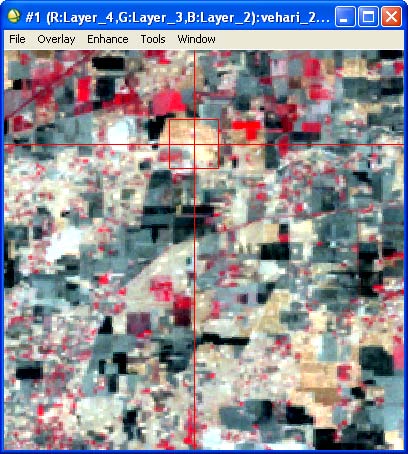
In this research paper Landsat ETM+ scene 2003 for the District Vehari (path 150, row 39) was used for hyperspectral image analysis. In order to use this scene, several steps were followed to prepare for an accurate extraction of vegetation endmember. These vital steps are: image registration, geometric correction, radiometric enhancement, and histogram equalization as discussed by Macleod and Congalton (1998), Mahmoodzadeh (2007) and Al-Awadhi et al., 2011. The scene was corrected and geo-referenced using projection UTM, zone 43 and datum WGS 84. Atmospheric correction operation was performed using ENVI software. Further, Minimum Noise Fraction (MNF), Pixel Purity Index (PPI), n-Dimensional Visualizer (n-DV) and Endmember Extraction technique has been used for hyperspectral image analysis (Figure 1).

The Pixel Purity Index (PPI) technique was adopted using ENVI 'automated spectral hourglass' application upon ETM+ image. The PPI was applied upon the full scene of the district. In this experiment 22,948,704 pixels were operated (Figure 3 The hyperspectral imaging, also known as imaging spectrometry, is now a reasonably familiar concept in the world of remote sensing. Hyperspectral images are spectrally providing ample spectral information (Shippert, 2003) to identify and distinguish between spectrally similar resource information. Consequently, hyperspectral imagery provides the potential for more accurate and detailed information extraction than is possible with other types of remotely sensed data (Shippert, 2004). Standard multispectral image processing techniques were generally developed to classify multispectral images into broad categories of surface condition. Hyperspectral imagery provides an opportunity for more detailed image analysis. Boardman (1993) and Boardman et al. (1995) were among the first to develop and commercialize a sequence of algorithms specifically designed to extract detailed information from hyperspectral imagery (Shippert, 2004). ENVI tools, applicable to a variety of applications, distinguish and identify the unique resource information present in the scene and map them throughout the image (Research System, Inc., 2004).

3. III. Results

The hyperspectral imaging is a new emerging technology in remote sensing which generates hundreds of images, at different wavelength channels, for the same area on the surface of the Earth (Goetz et al., 1985 A region from 0.38 to 2.5 ?m or 380 nm to 2500 nm using two hundred twenty four spectral channels, at nominal spectral resolution of 10 nm (González et al., 2010).

The Pixel Purity Index (PPI) is a new automated procedure in the hyperspectral analysis process (Boardman, 1993;Boardman et al., 1995) for defining potential image endmember spectra (Bateson and Curtiss, 1996) for spectral unmixing (Lillesand and Kiefer, 2000). When image spectra are treated as points in n-dimensional spectral space, endmember spectra should lie along the margins of the data cloud (MicroImages, Inc., 1999; Berman et al., 2004). The PPI creates a large number of randomly oriented test vectors anchored at the origin of the coordinate space. The spectral points are projected onto each test vector, and spectra within a threshold distance of the minimum and maximum projected values are flagged as extreme (Nascimento and Dias, 2005). As directions are tested, the process tallies the number of times an image cell is found to be extreme (Miao and Qi, 2007). Cells with high values in the resulting PPI raster should correspond primarily to 'edge' spectra . The PPI raster then can be used as a mask to control input to the n-dimensional visualizer (MicroImages, Inc., 1999; Zhang et al., 2008).

The most commonly used endmember extraction (Figure 5, 6 and Table 1, 2) tool is pixel purity index, which searches for vertices that define the data volume in n-dimensional space (Rogge et al., 2007). Commonly the first step of PPI is to apply MNF (Lee et al., 1990) to reduce the dimensionality of the data set (Green et al., 1988;Rogge et al., 2007). The MNF transform is used to determine the inherent dimensionality of image data, to segregate noise in the data, and to reduce the computational requirements for subsequent processing (Boardman and Kruse, 1994). The transformation based on an estimated noise covariance matrix, decorrelates and rescales the noise in the data (Research Systems, Inc., 2003;2004). This step results in transformed data in which the noise has unit variance and no band-to-band correlations. For the purposes of further spectral processing, the inherent dimensionality of the data is determined by examination of the final eigenvalues and the associated images. The data space can be divided into two parts: one part associated with large eigenvalues and coherent eigenimages, and a complementary part with near-unity eigenvalues and noise-dominated images. By using only the coherent portions, the noise is separated from the data, thus improving spectral processing results (Research Systems, Inc., 2001;2004).

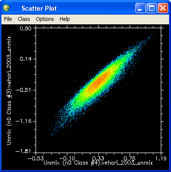
Spectra can be thought of as points in an ndimensional scatter plot, where n is the number of bands (Boardman et al., 1995). The coordinates of the points in n-space consist of 'n' values that are simply the spectral radiance or reflectance values in each band for a given pixel. The distribution of these points in n-space can be used to estimate the number of spectral endmembers and their pure spectral signatures (Research Systems, Inc., 2001). The scatter plot (Figure 7) is an important tool for exploring an image and helping to understand some of the spectral characteristics of features in an image. The two dimensional scatter plotting tool allows comparing not only the relationship between the data values in two selected bands but also the spatial distribution in the image of pixels in any area of the scatter plot. This combined functionality provides a very simple, twoband, interactive classification of image data (Research Systems, Inc., 2004).

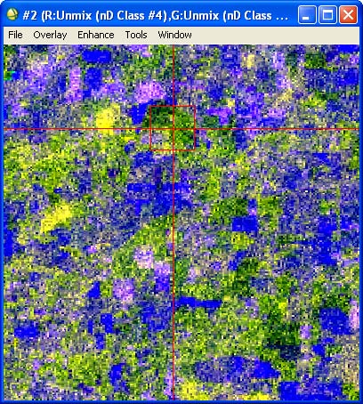
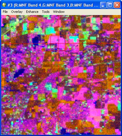
Spectral unmixing (Figure 9) algorithms (Lillesand and Kiefer, 2000; Rogge et al., 2006) use a variety of different statistical procedures to endmember extraction and estimate abundances. Unmixing problem comprises three sequential steps: dimension reduction, endmember determination, and inversion (Chang and Plaza, 2006). Because hyperspectral scenes can include extremely large amount of data, some algorithms for spectral unmixing first use image itself to estimate endmembers present in the scene. The dimension-reduction stage reduces the dimension of the original data in the scene (Cochrane, 2000;Mozaffar et al., 2008). The noise estimate can come from one of three sources; from the dark current image acquired with the data, from noise statistics calculated from the data (Richards and Jia, 1999), or from statistics saved from a previous transform. Both the eigenvalues and the Minimum Noise Fraction (MNF -Figure 10) images (eigenimages) are used to evaluate the dimensionality of the data (Qiu et al., 2006). Eigenvalues for bands that contain information will be an order of magnitude larger than those that contain only noise. The corresponding images will be spatially coherent, while the noise images will not contain any spatial information (Research Systems, Inc., 2004; Qiu et al., 2006). Processed by the author.

Processed by the author. The Mixture Tuned Matched Filtering (MTMF -Figure 11) algorithm builds upon the strengths of both matched filtering and spectral unmixing while avoiding the disadvantages of both (Boardman, 1998). Matched filtering performs partial unmixing and identifies abundance of spectral endmembers without knowing background endmember signatures (Harsanyi and Chang 1994; Boardman et al., 1995). Matched filtering does not distinguish rare spectral targets very well and assumes an additive signal based upon radio/radar applications. Spectral unmixing takes advantage of the hyperspectral leverage to solve the linear mixed pixel problem, but traditional spectral unmixing techniques require knowledge of all of the background endmembers (Boardman, 1993;Bateson and Curtiss, 1996;Bateson et al., 2000). Incorporating convex geometry concepts, mixtures must be non-negative and unit-sum helps identify false positives, unrealistic mixtures, and maps subpixel fractional abundances.

The Minimum Noise Fraction (MNF) data reduction transform and Mixture Tuned Matched Filtering (MTMF) partial unmixing classification algorithm are relatively new image processing techniques that have proven to be effective target detection tools (Research Systems, Inc., 2004). These techniques allow partial unmixing and subpixel target abundance estimation, products that cannot be achieved using spectral angle mapping algorithms (Mundt et al., 2007).

The n-dimensional visualizer serves as an interactive tool for multidimensional analysis and identification of spectral endmembers (Tompkins et al., 1997;Plaza et al., 2002). The data are displayed in a defined number of dimensions and spectral endmembers are identified as pixels that are located at the corner vertices (Tsai and Philpot, 1998). The ndimensional visualizer second round of spatial data reduction designed to identify particular pixels or group of pixels that represent the purest spectra within the image. These pure spectra are exported and saved as ROI's that can be used for subsequent image classification techniques.

The n-dimensional visualizer was used to interactively locate, identify, and cluster the most spectrally pure or unique pixels in the image by visualizing those pixels selected from the PPI as points in an multidimensional scatter plot (Figure 7), where the number of dimensions was defined by the total number of coherent MNF bands (Boardman, 1993;Harris, 2006). The advantage of the n-dimensional visualizer was that it allowed visualization of points in an n-dimensional space, forming a data 'cloud' (Berk et al., 1998;Harris, 2006).

Advantages of this technology include both the qualitative benefits derived from a visual overview, and more importantly, the quantitative abilities for systematic assessment and monitoring (Shippert, 2003) Pixel Purity Index Algorithm and N-Dimensional Visualization for ETM+ Image Analysis: A Case of District Vehari

4. IV. Discussion and Conclusions

The potential of hyperspectral remote sensing is exciting; there are special issues that arise with this unique type of imagery. For example, many hyperspectral analysis algorithms require accurate atmospheric corrections to be performed. To meet this need, sophisticated atmospheric correction algorithms have been developed to calculate concentrations of atmospheric gases directly from the detailed spectral information contained in the imagery (Roberts et al., 1993;Cochrane, 2000;Okin et al., 2001;Riano et al., 2002) itself without additional ancillary data. These corrections can be performed separately for each pixel because each pixel has a detailed spectrum associated with it. Several of these atmospheric correction algorithms are available within commercial image processing software (Shippert, 2004). However, several image analysis algorithms have been successfully used with uncorrected imagery (Shippert, 2003).

The MNF transform applied to the ETM+ data achieved a reasonable separation of coherent signal from complementary noise, therefore the MNF transformed eigenimages were employed and coupled with pixel purity index and n-dimensional visualization techniques to facilitate the extraction of the endmembers (Song, 2005;Qiu et al., 2006). After applying PPI thresholding, the data volume to be analyzed has been effectively reduced (Zhang et al., 2000). However, it is still possible that many less 'pure' pixels have crept in as candidate endmembers during the automatic selection process. All the pixels that were previously selected using the PPI thresholding procedure are displayed as pixel clouds in the ndimensional spectral space (Welch et al., 1998). To make possible the visualization of a scatter plot with more than two dimensions, the pixel clouds of high dimensions are cast on the two-dimensional display screen (Kruse et al., 1993;Tu et al., 1998). To effectively extract endmembers from high dimensional remote sensing data (Plaza et al., 2004) and to effectively process the data, it is often necessary that the dimensionality of the original data be decreased and noise in the data be segregated first, so the visualizing complexity and computational requirement for the subsequent analysis can be reduced (Kalluri et al., 2001;Qiu et al., 2006). This is often achieved through applying a minimum noise fraction transform to the high dimensional data (Qiu et al., 2006).

The hyperspectral sensors and analysis have provided more information from remotely sensed imagery than ever possible before. As new sensors provide more hyperspectral imagery and new image processing algorithms continue to be developed, hyperspectral imagery (Shippert, 2003) is positioned to become one of the most common research (Shippert, 2004) employed was implemented based on the comparison of a pixel spectrum with the spectra of known pure resource information, which can be effectively extracted using endmember selection procedures such as minimum noise fraction, pixel purity index and ndimensional visualization.

5. V. Acknowledgements

The

and 4) using Automated Hourglass Parameters: Number of MNF bands to use: 6 (excluding Thermal IR and Panchromatic); Number of PPI Iterations: 5,000; PPI Threshold Value: 2.500; Maximum number of PPI Pixels to use for Endmember Selection: 10,000; and Mapping Methods were selected: Mixture Tuned Matched Filtering (MTMF), Spectral Angle Mapper (SAM), andUnmixing. The Endmembers were selected for processing flow, a series of tools that use the spectrally over-determined nature of hyperspectral data to find the most spectrally pure or spectrally unique pixels within the dataset. This set of endmember signatures(Bateson and Curtiss, 1996;Bateson et al., 2000) was then used in the full range of mapping algorithms available in ENVI to determine locations, and in some cases subpixel abundances of endmembers(Harris, 2006). — Figure 1.

Figure 1 : Scheme for hyperspectral image analysis. — Figure 2. Figure 1 :

;González et al., 2010;Sánchez and Plaza, 2010). The concept of hyperspectral imaging originated at NASA's Jet Propulsion Laboratory in California, which developed instruments such as the Airborne Imaging Spectrometer (AIS), then called AVIRIS, for AirborneGlobal Journal of Human Social ScienceVolume XII Issue W XV Version I — Figure 3.

Figure 2 : District Vehari -Landsat ETM+ 2003 image. — Figure 4. Figure 2 :

Figure 3 : Showing the endmember pixels extracted by the PPI for the District Vehari. — Figure 5. Figure 3 :

Figure 4 : Showing Pixel Purity Index Plot for the District Vehari. — Figure 6. Figure 4 :

Figure 6 : Showing selected endmembers (MNF). — Figure 7. Figure 6 :

Figure 5 : Showing selected endmembers data. — Figure 8. Figure 5 :

Figure 7 : 2-D scatter plot applied upon unmixing using band X 4 and band Y 3. — Figure 9. Figure 7 :

. A Pixel Purity Index Algorithm and N-Dimensional Visualization for ETM+ Image Analysis: A Case of District Vehari considerable number of mixed pixels are present in any remotely sensed image (Mozaffar et al., 2008). Several research objectives were accomplished : ? Select optimal bands in hyperspectral images those are most useful in vegetation classification, ? Identify optimal endmember, signature spectrum that represents a certain class, for vegetation classification, and ? Test effective endmember extraction algorithms for classification of vegetation type. — Figure 10.

Figure 8 : Landsat ETM+, District Vehari. — Figure 11. Figure 8 :Figure 9 :

Figure 11 : Image showing mixture tuned matched filtering (MTMF). — Figure 12. Figure 11 :

Figure 13.

salinity (Ben-Dor et al., 2002). Vegetation scientists have

successfully used hyperspectral imagery to identify

vegetation species (Clark and Swayze, 1995), study

plant canopy chemistry (Aber and Martin, 1995;

Shippert, 2003), and detect vegetation stress.

a) Study Area

The District Vehari (Figure 2 and 8) lies between

29° 36' and 30° 22' North latitude and 71° 44' and 72° 53'

East longitude (GOP, 2000). The district is bounded on

the north by and Khanewal and Sahiwal, on the east by

Pakpattan, on the south by Bahawalpur and

Bahawalnagar, on the west by Lodhran and Khanewal.

endmembers being derived, and the number of endmembers,

estimated by an algorithm, with respect to the number of

spectral bands, and the number of pixels being processed,

also the required input data, and the kind of noise, if any, in

the signal model surveying done. Results of the present study

using the hyperspectral image analysis technique ascertain

that Landsat ETM+ data can be used to generate valuable

vegetative information for the District Vehari, Punjab Province,

Pakistan.

Note: The effectiveness of the hyperspectral image analysis technique used in this study lies in their ability to compare a pixel spectrum with the spectra of known pure vegetation, extracted from the spectral endmember selection procedures, including the reflectance calibration of Landsat ETM+ image using ENVI software, minimum noise fraction (MNF), pixel purity index (PPI), and n-dimensional visualization. The Endmember extraction is one of the most fundamental and crucial tasks in hyperspectral data exploitation, an ultimate goal of an endmember extraction algorithm is to find the purest form of spectrally distinct resource information of a scene. The endmember extraction tendency to the type

Figure 14. Table 1 :

Bands nD Class 1-2 nD Class 2-3 nD Class 3-4 nD Class 4-5 nD Class 5-6 nD Class 6-7 nD Class 7-8
1	81	74	75	84	74	76	76
2	68	62	62	84	61	64	66
3	78	66	67	99	69	74	75
4	70	57	68	77	71	86	64
5	255	103	255	48	255	255	109
8	1	255	255	38	1	1	255

Figure 15. Table 2 :

Bands nD Class 1-2 nD Class 2-3 nD Class 3-4 nD Class 4-5 nD Class 5-6 nD Class 6-7 nD Class 7-8
1	-45.668144	-9.559686	-13.362324	-42.251820	-40.435787	-43.774044	-11.297052
2	-3.265855	-0.914537	18.957897	-11.722809	3.940382	14.638547	4.918655
3	15.752277	-29.919695	-23.210220	-2.429869	20.311623	26.381514	-31.349176
4	296.551239	-137.255051	52.496872	-22.368624	294.801758	282.927765	-135.733566
5	-27.440727	146.126907	160.149399	-48.182602	-19.783876	-24.758867	136.516922
6	139.244019	-62.703640	27.703362	1.272109	137.308945	129.952774	-63.861103

Figure 16.

	purity index algorithm for remotely sensed
	hyperspectral image analysis, EURASIP Journal on
	Advances in Signal Processing, Vol. 2010, pp.1-13.
	doi: 10.1155/2010/969806.
	19. GOP (2000). District census report of Vehari 1998,
	Population Census Organization, Statistics Division,
	Government of Pakistan, Islamabad, Pakistan, p.1.
	20. Green AA, Berman M, Switzer P and Craig MD
	author wishes to thank his respected (1988). A transformation for ordering multispectral
	mentor Dr. Robert Bryant, Sheffield Centre for data in terms of image quality with implications for
	International Drylands Research, Department of noise removal, IEEE Transactions on Geoscience
	Geography, The University of Sheffield for review and and Remote Sensing, Vol. 26, pp.65-74.
Year	providing valuable comments on draft-version of this paper. 21. Green RO, Eastwood ML and Sarture CM (1998). Imaging spectroscopy and the airborne
2 30	References Références Referencias visible/infrared imaging spectrometer (AVIRIS),
Volume XII Issue W XV Version I	1. Aber JD and Martin ME (1995). High spectral resolution remote sensing of canopy chemistry, In: Summaries of the 5 th Annual JPL Airborne
D D D D ) A
(
Global Journal of Human Social Science	The spectral image processing system (SIPS) interactive visualization and analysis of imaging spectrometer data, Remote Sensing of Environment,

Appendix A

Appendix A.1

Appendix B

A method for manual endmember selection and spectral unmixing. A Bateson , B Curtiss . Remote Sensing of Environment 1996. 55 p. .
Endmember bundles: A new approach to incorporating endmember variability into spectral mixture analysis. A Bateson , G P Asner , C A Wessman . IEEE Transactions on Geoscience and Remote Sensing 2000. 38 (2) p. .
MODTRAN cloud and multiple scattering upgrades with application to AVIRIS. A Berk , L S Bernstein , G P Anderson , P K Acharya , D C Robertson , J H Chetwynd , Adler-Golden Sm . Remote Sensing of Environment 1998. 65 p. .
Acc essed on, asa.gov/pub/docs/workshops/95_docs/1.PDF. November 20, 2011.
Imaging spectrometry for Earth remote sensing. Afh Goetz , G Vane , J E Solomon , Rock Bn . 10.1126/science.228.4704.1147. Science 1985. 228 (4704) p. .
Spatial/spectral endmember extraction by multidimensional morphological operations. A Plaza , P Martinez , R Perez , J Plaza . IEEE Transactions on Geoscience and Remote Sensing 2002. 40 p. .
A quantitative and comparative analysis of endmember extraction algorithms from hyperspectral data. A Plaza , P Martinez , R Perez , J Plaza . IEEE Transactions on Geoscience and Remote Sensing 2004. 42 (3) p. .
B Zhang , X Wang , J Liu , L Zheng , Q Tong . Hyperspectral image processing and analysis system (HIPAS) and its applications, 2000. 66 p. .
FPGA implementation of the pixel p, C González , J Resano , D Mozos , A Plaza , D Valencia . ftp://popo.jpl.nasa.gov/pub/docs/worksho 2010. p. 6.
A fast iterative algorithm for implementation of pixel purity index. C I Chang , A Plaza . 10.1109/LGRS.2005.856701. IEEE Geoscience and Remote Sensing Letters 2006. 3 (1) p. .
A new growing method for simplex-based endmember extraction algorithm. C I Chang , C C Wu , W W Liu , Y C Ouyang . IEEE Transactions on Geoscience and Remote Sensing 2006. 44 p. .
Mapping minerals, amorphous materials, environmental materials, vegetation, water, ice, and snow, and other materials: The USGS Tricorder Algorithm. Clark Rn , G A Swayze . Summaries of the 5th Annual JPL Airborne Geoscience Workshop, 1995. p. .
, C O Boulder , Url . http://www.ittvis.com November 28, 2011.
Spectral mixture analysis for subpixel vegetation fractions in the urban environment: How to incorporate endmember variability. C Song . Remote Sensing of Environment 2005. 95 p. .
Green vegetation, non-photosynthetic vegetation, and soils in AVIRIS data. D A Roberts , Smith Mo , J B Adams . Remote Sensing of Environment 1993. 44 p. .
Iterative spectral unmixing for optimizing per-pixel endmember sets. D M Rogge , B Rivard , J Zhang , J Feng . IEEE Transactions on Geoscience and Remote Sensing 2006. 44 p. .
Integration of spatial-spectral information for the improved extraction of endmembers. D M Rogge , B Rivard , J Zhang , A Sanchez , Harris J Feng , J . Remote Sensing of Environment 2007. 110 p. .
Earth Resources Observation and Science Center. http://glovis.usgs.gov/ USGS 2008. Accessed on December 04. 2008.
Mapping of several soil properties using DAIS-7915 hyperspectral scanner data: A case study over clayey soils in Israel. E Ben-Dor , K Patkin , A Banin , A Karnieli . 10.1080/01431160010006962. International Journal of Remote Sensing 2002. 23 (6) p. .
Exploring ENVI, Hyperion images, URL:www.isprs.org/proceeding 2004. Research System, Inc.
Spectral analysis of ASTER data covering part of the Neoproterozoic Allaqi-Heiani suture, Southern Egypt. F Qiu , M Abdelsalam , P Thakkar . Journal of African Earth Sciences 2006. 44 p. .
Derivative analysis of hyperspectral data. F Tsai , W Philpot . Remote Sensing of Environment 1998. 66 p. .
, Geoscience Workshop . http://www.isprs.orgdf 2011. Oman. 10 p. . (Assessed on September)
Practical limits on hyperspectral vegetation discrimination in arid and semiarid environments. G S Okin , D A Roberts , B Burray , W J Okin . Remote Sensing of Environment 2001. 77 p. .
Pixel purity index and masking aid endmember selection, TNTmips, Inc Microimages . V6.10. http://www.microimages.com/documentation/TechGuides/61Ppi.pdf.(Accessedon 1999. November 28, 2 011.
Remote sensing digital image analysis: An Introduction, Third Edition, J A Richards , X Jia . 1999. Berlin: Springer-Verlag. p. .
Vertex component analysis: A fast algorithm to unmix hyperspectral data. Jmp Nascimento , Jmb Dias . 10.1109/TGRS.2005.844293. IEEE Transactions on Geoscience and Remote Sensing 2005. 43 (4) p. .
Partial unmixing of hyperspectral imagery: Theory and methods. J T Mundt , D R Streutker , N F Glenn . http://www.asprs.org/a/publications/proceedings/tampa2007/0046.pdf.(Accessedon Paper in ASPRS Annual Conference, (Tampa, Florida
) 2007. May 7-11, 2007. November 28. 2011.
Automating spectral unmixing of AVIRIS data using convex geometry concepts. J W Boardman . ftp://popo.jpl.nasa.gov/pub/docs/workshops/93_docs/4.PDF.(Accessedon Summaries of the 4 th Annual JPL Airborne Geoscience Workshop, 1993. November 19. 2011. p. .
Automated spectral analysis: A geologic example using AVIRIS data, north Grapevine Mountains. J W Boardman , F A Kruse . Proceedings of 10thThematic Conference on Geologic Remote Sensing, (10thThematic Conference on Geologic Remote SensingNevada; Ann Arbor, MI
) 1994. I p. . Environmental Research Institute of Michigan
Mapping target signatures via partial unmixing of AVIRIS data. J W Boardman , F A Kruse , R O Green . http://trs-new.jpl.nasa.gov/dspace/bitstream/2014/33635/1/94-1613.pdf Summaries of the 5th Annual JPL Airborne Geoscience Workshop, 1995. November 19. 201 1. p. .
Leveraging the high dimensionality of AVIRIS data for improved sub-pixel target unmixing and rejection of false positives: Mixture Tuned Matched Filtering. J W Boardman . Summaries of the 7th Annual JPL Airborne Geoscience Workshop, ps/98_docs/8.pdf. (Accessed on, 1998. November 28, 201 1.
The successive projection algorithm (SPA), an algorithm with a spatial constraint for the automatic search of endmembers in hyperspectral data. J Zhang , B Rivard , D M Rogge . Sensors 2008. 8 p. .
Endmember extraction from highly mixed data using minimum volume constrained nonnegative matrix factorization. L Miao , H Qi . IEEE Transactions on Geoscience and Remote Sensing 2007. 45 p. .
Using vegetation reflectance variability for species level classification of hyperspectral data. M A Cochrane . International Journal of Remote Sensing 2000. 21 (10) p. .
ICE: An automated statistical approach to identifying endmembers in hyperspectral images. M Berman , H Kiiveri , R Lagerstrom , A Ernst , R Dunne , J Huntington . IEEE Transactions on Geoscience and Remote Sensing 2004. 42 p. .
Vegetation endmember extraction in s/XXXVII/congress/7_pdf/3.../34.pdf, M H Mozaffar , Mjv Zoej , M R Sahebi , Y Rezaei . 2008. November 20, 2011.
Introduction to hyperspectral al.ohio.edu/pdf/shippert.pdf, P Shippert . 2003. 2011. 20.
Why use hyperspectral imagery? Photogrammetric Engineering & Remote Sensing, ~mignotte/IFT6150/ComplementCours/Hyperspectr alImagery.pdf. (Accessed on, P Shippert . 2004. November 20, 2011.
Considerations in collecting, processing, and analyzing high spatial resolution hyperspectral data for environmental investigations. R J Aspinall , Marcus Wa , J W Boardman . Journal of Geographical Systems 2002. 4 p. .
ASTER as a source for topographic data in the late 1990's. R Welch , T Jordan , Lang H Murakami , H . IEEE Transactions on Geoscience and Remote Sensing 1998. 36 p. .
Utilization of Landsat ETM+ data for mineral-occurrences mapping over Dalma and Dhanjori. S K Pal , T J Majumdar , A K Bhattacharya , R Bhattacharyya . International Journal of Remote Sensing 2011. 32 (14) p. . (: An advanced spectral analysis approach)
GPU implementation of the pixel purity index algorithm for hyperspectral people/aplaza/Papers/Conferences/2010.Cluster.GP U.pdf, S Sánchez , A Plaza . 2010. November 20, 2011.
Optimization of endmembers for spectral mixture analysis. S Tompkins , J F Mustard , C M Pieters , D W Forsyth . Remote Sensing of Environment 1997. 59 p. .
The use of remote sensing & geographical information systems to identify vegetation: The case of, T Al-Awadhi , Al-Shukili A , Al-Amri Q . Dhofar/proceedings/2011/ISRSE34/211104015Final00239.p 2011.
A noise subspace projection approach to target signature detection and extraction in an unknown background for hyperspectral images. T Tu , Chen C Chang , C . IEEE Transactions on Geoscience and Remote Sensing 1998. 36 (1) p. .

Pixel Purity Index Algorithm and n-Dimensional Visualization for ETM+ Image Analysis: A Case of District Vehari

Table of contents